
42. Recomputation
This chapter demonstrates recomputation as the most essential technique for efficient search in Gecode. It is highly recommended to read Hybrid recomputation before reading this chapter.
Overview. The simplest possible search engine based on recomputation, where all spaces needed for search are recomputed from the root of the search tree, is discussed in Full recomputation. Important invariants for recomputation and how they must be taken into account by search engines using recomputation are discussed in Recomputation invariants. How best solution search is combined with recomputation is discussed in Branch-and-bound search. The following three sections present important optimizations for search engines using recomputation: Last alternative optimization shows how last alternative optimization can avoid commit() operations during recomputation; Hybrid recomputation shows how hybrid recomputation that stores additional spaces can be used to speed up search; Adaptive recomputation shows adaptive recomputation that helps speeding up search in case of failures.
Important
All sections in this chapter make the simplifying assumption that choices are binary, dealing with non binary choices is similar to Depth-first search. The search engine in An example engine combines all recomputation techniques of this chapter for the general case.
42.1. Full recomputation
This section demonstrates search based on full recomputation. While full recomputation is unrealistic, the search engine presented here helps in understanding the ideas behind recomputation. In particular, the search engine serves as an example for important invariants for recomputation that are discussed in Recomputation invariants.
Search engine.
...
// [dfs using full recomputation:edge class]

Space* dfs(Space* s, Space* r, Edge* p) {
  switch (s->status()) {
  ...
  case SS_BRANCH:
    {
      // [dfs using full recomputation:explore first alternative]
      // [dfs using full recomputation:explore second alternative]
    }
  }
}

Space* dfs(Space* s) {
  if (s->status() == SS_FAILED) {
    delete s; return NULL;
  }
  Space* r = s->clone();
  Space* t = dfs(s,r,NULL);
  delete r;
  return t;
}
Download: dfs-using-full-recomputation.cpp
Program 42.1 shows the outline for the search engine that implements depth-first search with full recomputation. The function dfs() that takes a single space s as its argument is called by the user, the function dfs() that takes three arguments implements exploration with full recomputation.
The basic idea of the search engine is to always keep a single space r as the root space of the search tree to be explored. Exploration maintains a current space and a path consisting of edges that defines which node in the search tree is currently being explored. Exploration is governed by the invariant that the current space can always be recomputed from the path of edges maintained by the search engine.
Initially, when the user calls the dfs() function taking a single argument, the root space r is computed as a clone of the space s passed as argument. As only stable and non-failed spaces can be cloned (see Space-based search), the status() function is used to find out whether propagation on s results in failure. If not, the root space r is created as a clone of s and the search engine dfs() is called with s as the current space, r as the root space, and NULL as the current path from the current space to the root space.
Edges for recomputation.
class Edge {
protected:
  Edge* p;
  const Choice* ch;
  unsigned int a;
public:
  Edge(Space* s, Edge* e)
    : p(e), ch(s->choice()), a(0) {}
  // [dfs using full recomputation:next alternative]
  // [dfs using full recomputation:committing a space]
  // [dfs using full recomputation:recomputing a space]
  ~Edge(void) {
    delete ch;
  }
};
Program 42.2 shows the class Edge implementing an edge of a path to be used for recomputation. The class stores a pointer p to the predecessor edge, a choice ch, and the number of the alternative a that corresponds to the edge. Edges are organized from the current node (space) of the search tree upwards to the root: the last edge of a path connects to the root of the search tree and has NULL as its predecessor p. Note that we restrict our attention in this chapter to binary choices only.
Initialization by the Edge’s constructor takes the current space of the search engine s and the predecessor edge e and initializes the edge with the choice for s and the first alternative. Deleting an edge also deletes the stored choice ch.
An edge provides a next() function that redirects the edge to the next alternative:
  void next(void) {
    a++;
  }
The commit() function of an edge commits a space s to the alternative that corresponds to the edge:
  Space* commit(Space* s) const {
    s->commit(*ch,a); return s;
  }
The function returns the space just for convenience as can be seen below.
Finally, recomputing a space corresponding to an entire path of edges is implemented by the recompute() function. The function takes the root space r as argument and is implemented as follows:
  Space* recompute(Space* r) const {
    return commit((p == NULL) ? r->clone() : p->recompute(r));
  }
First, the function traverses the path of edges upwards until the root of the path is reached. Then it creates a clone of the root space r and performs the commit() operations for each edge on the path.
Exploring alternatives. The central invariant that the current path of edges p must always correspond to the current space is essential for how the search engine implementing full recomputation explores the search tree.
Before exploring the first alternative recursively, a new edge is created for the first alternative, the current space s is committed to the first alternative, and exploration continues recursively:
      Edge e(s,p);
      if (Space* t = dfs(e.commit(s),r,&e))
        return t;
Note that all resource management for handling edges is done automatically: as soon as the edge e goes out of scope, it is automatically deleted (and hence also the choice for the edge is deleted).
Again, exploration of the second alternative maintains the central invariant: the edge is redirected to the next alternative and then a space corresponding to the path of edges is recomputed:
      e.next();
      return dfs(e.recompute(r),r,&e);
Cost of recomputation. It is important to notice the following facts about the cost of recomputation, where we compare the search engine using full recomputation to the search engine without recomputation in Binary depth-first search:
While the number of
commit()operations on spaces drastically increases for full recomputation, the number ofstatus()operations executed remains exactly the same.However, execution of
status()during recomputation is more expensive as more constraint propagation needs to be done: full recomputation always starts from the root space where only little constraint propagation has been performed.The number of
clone()operations executed by full recomputation is never larger than the number ofclone()operations without recomputation.Typically, the number of
clone()operations is much smaller: recomputation is optimistic in the sense that a clone is created and recomputation is performed only if a node is required for exploration. A search engine without recomputation is pessimistic in that it always creates a clone before continuing exploration to be able to backtrack to a space that might be required for further exploration.Hybrid recomputation presents hybrid recomputation as a technique that makes recomputation less optimistic in that it creates more clones before continuing exploration. Adaptive recomputation presents adaptive recomputation that makes recomputation even less optimistic in cases where it is likely that exploration can benefit from additional clones.
A detailed evaluation of recomputation in Gecode and a comparison to other techniques for implementing search can be found in [42]. An evaluation of different recomputation techniques (although in a different setup) can be found in [46] and [47].
42.2. Recomputation invariants
This section discusses two important invariants that govern recomputation. The first invariant is that recomputation can only use compatible choices for commit operations: the notion of choice compatibility has been sketched in Space-based search and is detailed in Choice compatibility. The second invariant is concerned with the fact that recomputation is not always deterministic. However, Recomputation is not deterministic explains why recomputation still works even though it is not deterministic.
42.2.1. Choice compatibility
Space-based search introduced the notion that a space s is compatible with a choice ch (that is, ch can be used for a commit() operation on s). For recomputation, a more general notion of compatibility is needed: during recomputation, a search engine performs commit() operations using choices that have been computed earlier on a path in the search tree.
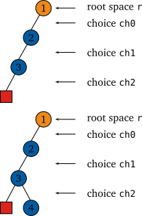
Figure 42.1 Example situations during recomputation
Consider the situation sketched in the left part of Figure 42.1 with a root space r and choices ch0, ch1, and ch2 as stored on the path of edges for recomputation. That is, all choices have been computed by the choice() function from a clone of the root space r where in between the calls to choice() other operations on the space have been performed. For example, the search engine implementing full recomputation from Full recomputation has executed the status() and commit() functions several times in order to compute the choices.
Suppose that s is a clone of r (computed by s=r->clone()). Then all choices are compatible with s. Now suppose that t is a clone of s. Then all choices are still compatible with t. Hence, if a choice ch has been created for a space r all spaces that are related by cloning to r are compatible with ch. Compatibility continues to hold even if other operations (such as commit() operations for other choices, computing the status of a space, or the creation of new variables, propagators, and branchers) are performed on a space that is clone-related. The only exception is the choice() function of a space.
Suppose that recomputation proceeds by recomputing the space s for node 4 as shown in the right part of Figure 42.1. Assume that s requires branching. Hence, a search engine is executing s->choice(). After executing the choice() function, all previous choices ch0, ch1, and ch2 are not any longer compatible with s.
Order of commit() operations. The choices ch0, ch1, and ch2 do not have to be used for commit() in the same order in which they have been created. However, it is more efficient to use them in the order ch0, ch1, and ch2. The difference is that if a space has \(n\) branchers and the choices correspond to different branchers, then a commit() operation uses \(O(1)\) time to find the corresponding brancher for a choice if the choices are used in order. If they are not used in order, a commit() operation uses \(O(n)\) time to find the corresponding brancher. Having said all that, \(n\) is typically just one or two.
42.2.2. Recomputation is not deterministic
Assume that a search engine has recorded a path from a node in the search tree and that the space s corresponds to that node in the tree. Then, when a space t for that node is recomputed, the two spaces s and t might actually differ: the amount of propagation performed by s and t can be different.
The difference in propagation is due to the fact that Gecode supports propagators that are weakly monotonic but not necessarily monotonic. In summary, a weakly monotonic propagator can perform more or less propagation (that is, prune more values from variables domains or prune fewer values from variable domains) but is still correct and checking, see also Weakly monotonic propagators..
As weakly monotonic constraint propagation is still correct and checking, also recomputation is correct in the following sense: All solutions that are found by search starting from space s are also found by search starting from space t. However, search might find the solutions in different order when starting from either s or t.
Consider the special case that s is failed. The recomputed space t might not necessarily be failed. That is, s performed more constraint propagation than t. However, additional search from t will never find any solution. The same is also true with the roles of s and t exchanged: even though s is not failed, the recomputed space t can be failed.
For search engines using recomputation this typically does not pose any problems. In most cases, a search engine does not attempt to recompute a space that it assumes to be non-failed. Consider the depth-first search engine using full recomputation from Full recomputation. There, the spaces that are recomputed correspond to nodes in the search tree not yet explored. In other words, when recomputing spaces that have been explored previously, a search engine cannot make the assumption that the space is not failed just because the space explored previously has not been failed.
An exception is adaptive recomputation to be discussed in Adaptive recomputation as an optimization for recomputation. Adaptive recomputation recomputes previously explored spaces to speed up further search.
For a detailed discussion of weakly monotonic propagation together with the consequences for search including recomputation, please consult [53].
42.3. Branch-and-bound search
The first idea to combine recomputation with best solution search is to take the engine for best solution search without recomputation (see Branch-and-bound search) and add recomputation to it along the lines of Full recomputation. A search engine implementing this approach would work roughly as follows: recompute a space and, if needed, add the constraints to the space such that the space can only lead to a better solution.
A tighter integration of recomputation and best solution search is in fact much better: instead of adding the constraints for a better solution to the space that is recomputed, add it to the space from which recomputation starts (with full recomputation: the root space). The advantage is that if adding the constraints to the space from which recomputation starts already leads to failure, the entire subtree starting from that space can be discarded (with full recomputation: search is done).
...
void bab(Space* s, Space*& r, Space*& b, Edge* p) {
  switch (s->status()) {
  ...
  case SS_SOLVED:
    // [bab using full recomputation:solved]
  case SS_BRANCH:
    {
      ...
      // [bab using full recomputation:explore second alternative]
    }
  }
}

Space* bab(Space* s) {
  ...
  Space* r = s->clone();
  Space* b = NULL;
  bab(s,r,b,NULL);
  ...
}
Download: bab-using-full-recomputation.cpp
Program 42.3 sketches branch-and-bound best solution search using full recomputation. The search engine takes the current space s, the root space r, the so-far best solution b, and the predecessor edge p as arguments. Note that both the root space r and the so-far best solution b are passed by reference as they change during exploration.
When the search engine finds a new solution s, it replaces the so-far best solution b by s and updates the root space by adding the constraints that r must yield better solutions than b as follows:
    delete b;
    (void) s->choice(); b = s->clone(); delete s;
    r->constrain(*b);
    if (r->status() == SS_FAILED) {
      delete r; r = NULL;
    } else {
      Space* c = r->clone(); delete r; r = c;
    }
    break;
The root space then must be checked for failure. If the root space is failed, it is deleted and the pointer to the root space becomes NULL. Otherwise, the root space becomes a clone of the newly computed space to save memory (as mentioned earlier, it is better to store a pristine clone of a space than a space on which propagation has been performed).
Exploring the second alternative of a choice checks whether the root space is already failed:
      if (r != NULL)
        bab(e.recompute(r),r,b,&e);
42.4. Last alternative optimization
This section presents an important optimization for recomputation that helps to avoid many commit operations during recomputation. Even though the optimization is discussed in the context of full recomputation, it is applicable to all situations in which recomputation is used.
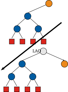
Figure 42.2 Last alternative optimization (LAO)
Consider a situation during search as shown in the left part of Figure 42.2. There, the entire left subtree emanating from the root node (colored in orange) has been explored. When exploration continues for the right subtree, each time a node is recomputed, a clone of the root node is made immediately followed by a commit operation for the second alternative. Hence it is much better to compute a new root node for the entire right subtree and perform the corresponding commit operation just once. This optimization is referred to as last alternative optimization (LAO) [47]. Figure 42.2 shows the new root of the search tree after performing LAO. Note that no space needs to be stored for the previous root node as it will never be used again for recomputation.
...
class Edge {
...
  // [dfs using full recomputation and lao:test for last alternative]
  ...
};

Space* dfs(Space* s, Space*& r, Edge* p) {
  switch (s->status()) {
  ...
  case SS_BRANCH:
    {
      Edge e(s,p);
      if (Space* t = dfs(e.commit(s),r,&e))
        return t;
      e.next();
      // [dfs using full recomputation and lao:perform lao]
      return dfs(e.recompute(r),r,&e);
    }
  }
}
...
Download: dfs-using-full-recomputation-and-lao.cpp
Program 42.4 shows a search engine implementing left-most depth-first search using full recomputation and LAO. Only very few aspects have changed compared to the engine for full recomputation without LAO from Full recomputation. An important change is that the root space is now passed by reference: this is necessary as the root space changes during exploration.
The Edge class is extended by a function la() that tests whether an edge happens to be a last alternative:
  bool la(void) const {
    return (p == NULL) && (a == 1);
  }
The actual optimization is performed just before exploring the second alternative:
      if (e.la()) {
        Space* t = r;
        if (e.commit(t)->status() == SS_FAILED)
          return NULL;
        r = t->clone();
        return dfs(t,r,NULL);
      }
The space t serves as a temporary reference. After performing the commit() operation on t for the second alternative, it is tested whether the new root node is already failed. The new root space becomes the clone of t: this is important as a clone typically requires less memory than a space on which constraint propagation has been performed (see Binary depth-first search).
42.5. Hybrid recomputation
Exploration based on copying alone or based on full recomputation is unrealistic. As already described in Hybrid recomputation, Gecode’s search engines use hybrid recomputation: they create a clone now and then to limit the amount of recomputation.
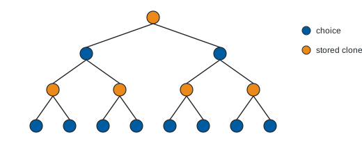
This section describes hybrid recomputation where the amount of recomputation is limited by the commit distance \(c_d\): during recomputation at most \(c_d\) commit() operations are executed. Hybrid recomputation with commit distance \(c_d=2\) where orange nodes are nodes that store a clone is shown below.
...
const unsigned int c_d = 5;

class Edge {
protected:
  ...
  Space* c;
public:
  Edge(Space* s, Edge* e)
    : p(e), ch(s->choice()), a(0), c(NULL) {}
  ...
  // [dfs using hybrid recomputation:create clone]
  // [dfs using hybrid recomputation:perform recomputation]
  ...
};

Space* dfs(Space* s, Edge* p, unsigned int d) {
  switch (s->status()) {
  ...
  case SS_BRANCH:
    {
      // [dfs using hybrid recomputation:store clone if needed]
      // [dfs using hybrid recomputation:explore first alternative]
      ...
    }
  }
}

Space* dfs(Space* s) {
  return dfs(s,NULL,c_d);
}
Download: dfs-using-hybrid-recomputation.cpp
The additional clones are stored in a field c in the Edge class shown in Program 42.5. Initially, the field c does not store a clone. The intuition is that the clone c (if not NULL) is a clone that corresponds to the node to which the edge leads (please remember that edges lead upwards to the root of the search tree).
The function clone() stores a clone of a space s in an edge:
  void clone(Space* s) {
    c = s->clone();
  }
Recomputation as performed by the recompute() function now continues to search the path of edges until an edge that stores a clone is found:
  Space* recompute(void) const {
    return commit((c != NULL) ? c->clone() : p->recompute());
  }
It must be guaranteed that there is always at least one edge in a path that stores a clone, otherwise recomputation would crash (see below).
The function dfs() that implements exploration takes the additional argument d (for distance) which defines how many commit() operations would be needed to recompute the current space. If d reaches the limit c_d (for simplicity, c_d is a constant as defined in Program 42.5), a new clone must be stored in the current edge. Hence, the code for branching starts by checking whether a clone must be stored for the current edge e:
      Edge e(s,p);
      if (d >= c_d) {
        e.clone(s); d=0;
      }
The initial call to the function dfs() that implements exploration takes c_d as value for d. By this, it is guaranteed that the first edge stores a clone (that is, a clone that corresponds to the root node of the search tree).
Exploring the alternatives is as before, the only change is that the incremented distance d+1 is passed as additional argument:
      if (Space* t = dfs(e.commit(s),&e,d+1))
        return t;
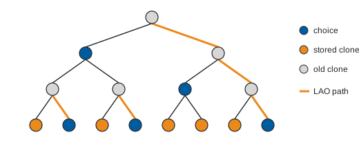
LAO as described for full recomputation (Last alternative optimization) can be added analogously to hybrid recomputation. Therefore we do not present hybrid recomputation with LAO. However, how LAO performs with hybrid recomputation is shown below: gray nodes correspond to nodes where a clone had been stored, while orange nodes correspond to nodes where a clone has been moved due to LAO.
42.6. Adaptive recomputation
Consider the situation when a search engine using recomputation encounters a failed space during exploration. Then it is quite likely that as exploration continues, more failed spaces are found during search. This is due to the fact that some decision made during branching (that is, some alternative) has lead to failure. It is quite likely that the wrong decision from which search must recover is somewhere on the path to the root node.
That means that search now must explore the entire subtree starting from the wrong decision. In this situation it would be advantageous if additional clones were available for exploring the entire subtree. With other words, after encountering failure, search should become more pessimistic by investing into the creation of additional clones to speed up further exploration.
Adaptive recomputation [47] optimizes recomputation in the case of failures: an additional clone is created during recomputation. The idea is that on a path of length \(n\) without any clone, an additional clone is placed in the middle of that path. This additional clone then speeds up further recomputation (which is likely to occur as has been argued above).
Adaptive recomputation is controlled by a parameter called adaptive distance \(a_d\): only if \(n\geq a_d\) an additional clone is created. This avoids creating an excessive amount of clones.
...
const unsigned int c_d = 5;
const unsigned int a_d = 2;

class Edge {
protected:
  ...
  Space* recompute(unsigned int n, unsigned int& d) {
    if (c != NULL) {
      d = (n >= a_d) ? n/2 : n;
      return commit(c->clone());
    } else {
      Space* s = p->recompute(n+1,d);
      if ((d == n) && (s->status() != SS_FAILED))
        clone(s);
      return commit(s);
    }
  }
  Space* recompute(unsigned int& d) {
    return recompute(1,d);
  }
  ...
};

...
Download: dfs-using-adaptive-recomputation.cpp
Adaptive recomputation is sketched in Program 42.6. The only change compared to hybrid recomputation (see Hybrid recomputation) is the implementation of recompute(). The argument n is the length of the path to the next clone. When a clone is found, d is set to \(\lfloor \frac{\mathtt n}{2}\rfloor\) provided that \(\mathtt{n}\geq\mathtt{a\_d}\). Otherwise d is set to n (its old value) which also prevents that an additional clone is created. For the edge that is d commit() operations away from the current space, a new clone is stored on the path, provided that the space s is not failed.
The space s can be failed as has been discussed in Recomputation is not deterministic. The search engine here takes a rather simplistic approach to this situation: it just does not store a clone. A real-life engine would take more benefit from the information that a space on the path is actually failed: it would immediately discard the entire path below the failed space, see An example engine.
Another optimization that a real-life search engine would employ is to not place a clone in a position where it could be moved by last alternative optimization, see again An example engine.