22. Crossword puzzle

This chapter studies solving crossword puzzles and presents a simple model using nothing but distinct and element constraints.

The simple model for this classical problem is shown to work quite well compared to a constraint-based approach to solving crossword puzzles using a dedicated problem-specific constraint solver  [1] . This underlines that an efficient general-purpose constraint programming system actually can go a long way.

22.1. Problem

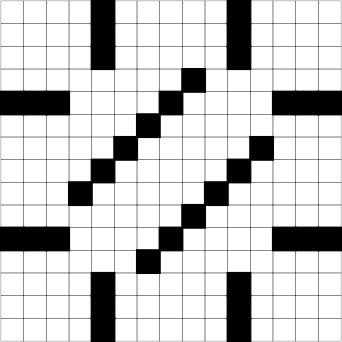
Figure 22.1 A crossword puzzle grid

To solve a crossword puzzle problem, a crossword grid (see Figure 22.1 for an example) must be filled with words (from a predefined dictionary) extending both in horizontal and vertical directions such that:

• If words cross at a field of the grid, the words’ letters at the crossing field are the same.

• No word is used twice.

Words use lowercase letters only and extend as far as they can. That is, the beginning (and the end) of a word must either be adjacent to a black field on the grid or must be a field on the grid’s border.

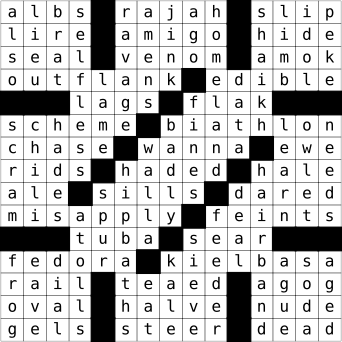
Figure 22.2 Solution for crossword puzzle grid from Figure 22.1

An example solution for the grid from Figure 22.1 is shown in Figure 22.2 .

22.2. Model

The model uses two sets of variables:

• The model uses for each word on the grid a word variable. A value for a word variable is a dictionary index defining the index of the word chosen from the dictionary of all words.

  The script for the model uses the word variables only as temporary variables for posting constraints. To simplify posting constraints, words are processed in groups of words of the same length. In particular, dictionary indices are also defined with respect to words of the same length in the dictionary.

• For each field on the grid, the model uses a letter variable. The values for a letter variable are either 0 (for a black field on the grid) or a character code between ’a’ and ’z’ for lowercase letters.

Given the sets of variables, the constraints for the model are straightforward:

• All word variables for words of the same length must be distinct. Only word variables for words of the same length need to be constrained to be distinct, as words of different length are distinct by definition.

• Assume that \(w\) is a word variable for a word of length \(n\) on the grid and \(x_0,\ldots, x_{n-1}\) are the letter variables that correspond to the word on the grid. Assume further that \(0\leq p<n\) and that an array \(\mathtt{w2l}\) (for word to letter) maps the dictionary indices of all words of length \(n\) to their \(p\)-th letter. Then, the letter variable \(x_p\) can be linked to the word variable \(w\) by posting the constraint that \(\mathtt{w2l}_w=x_p\) (this is an element constraint).

Program 22.1 Crossword script

...
// [crossword:grid specification]

...
// [crossword:words specification]
class Crossword : public Script {
protected:
  const int w, h;
  IntVarArray letters;
public:
  Crossword(const Options& opt)
    : Script(opt), w(grid[0]), h(grid[1]),
      letters(*this,w*h,'a','z') {
    // [crossword:set up]
    // [crossword:initialize black fields]
    // [crossword:process words by length]
    // [crossword:branching]
  }
  // [crossword:print function]
  ...
};

...

Download: crossword.cpp

An outline for the script implementing the crossword puzzle is shown in Crossword script . The script stores the width w and the height h of the grid and an integer variable array letters for the letter variables (including the black fields). The values for letters range from ’a’ to ’z’ (black fields are discussed below).

22.2.1. Grid and words specification.

Program 22.2 Grid and words specification

const int grid[] = {
  // Width and height of crossword grid
  15, 15,
  // Number of black fields
  36,
  // Black field coordinates
  0,4, 0,10, 1,4, 1,10, 2,4, 2,10, 3,8, 4,0, 4,1, 
  ...
  // Length and number of words of that length
  8, 8,
  // Coordinates where words start and direction (0 = horizontal)
  0,3,0, 0,9,0, 3,0,1, 5,7,1, 7,5,0, 7,11,0, 9,0,1, 11,7,1, 
  ...
  // End marker
  0
};

const int n_words[] = {
  1, 26, 66, 633, 2443, 4763, 7585, 10380, 10974
};
const char** words[] = {
  ...
};

The specification for the grid used in this case study (see More information for more information) and the word dictionary are shown in Grid and words specification. . The grid specification contains information about the dimension of the grid (as used in Crossword script ), the number and coordinates of black fields on the grid, and the start coordinates of words and their direction on the grid for each word length permitted by the grid.

For each word length \(l\), the array \(\mathtt{n_words}_l\) defines how many words of length \(l\) exist in the dictionary of words. That is, for a word length \(l\), the set of dictionary indices is \(\{0,\ldots,\mathtt{n_words}_l-1\}\). The array words provides access to the letters of a word of some given length with a given dictionary index. That is, for a given word length \(l\) and for a position in the word \(p\) with \(0\leq p<l\), \(\mathtt{words}_{l,i,p}\) (or \(\mathtt{words}[l][i][p]\) in C++) is the \(p\)-th letter of the word with dictionary index \(i\) among all words of length \(l\) (where \(0\leq i<\mathtt{n_words}_l\)) in the dictionary. The dictionary of words just contains words of length at most eight as this is sufficient for the example grid used in this case study.

The word list is based on SCOWL-55 (Spell Checking Oriented Word Lists) truncated to words of length at most eight, see wordlist.sourceforge.net . Please check the source file available from Crossword script for copyright information.

22.2.2. Grid initialization.

The grid specification is accessed by the pointer g (with the width and height part already skipped). The matrix ml (see Matrix interface for arrays ) supports access to the letters as a matrix:

    const int* g = &grid[2];
    Matrix<IntVarArray> ml(letters, w, h);

The black fields of the grid are initialized by storing a variable black at the respective coordinates:

    IntVar black(*this,0,0);
    for (int n = *g++; n--; ) {
      int x=*g++, y=*g++; ml(x,y)=black;
    }

At first sight, the treatment of black fields in the grid appears to be inefficient. First, each element in the integer variable array letters is initialized (in the initialization list of the constructor Crossword()) to a new integer variable with values ranging from ’a’ to ’z’. Then, some variables become redundant as their fields are overwritten by black. However, this only matters initially when a space of class Crossword is created. As soon as a clone of that space is created, the redundant variables are not copied and hence do not matter any longer. Moreover, all black fields on the grid share a single variable black which saves memory compared to a variable for each black field on the grid.

22.2.3. Processing words by length.

As suggested by the grid specification, words are processed in groups of the same length. The loop that processes all words of the same length l has the following structure:

    while (int l = *g++) {
      int n = *g++;
      // [crossword:initialize array of words]
      // [crossword:process word on grid]
    }

Here, n is initialized to the number of words with length l in the grid.

To enforce that all n words of the same length l are distinct, an integer argument array wosl (for words of same length) is created (see Integer and Boolean variable arrays ), where each variable takes the possible dictionary indices for words of length l as values. The word variables in wosl are constrained to be distinct as follows:

      IntVarArgs wosl(*this,n,0,n_words[l]-1);
      distinct(*this, wosl);

22.2.4. Constraining letters by words.

The remaining constraints link a word variable to the variables for its letters. All words of length l are processed as follows:

      IntArgs w2l(n_words[l]);
      for (int i=0; i<n; i++) {
        int x = *g++, y = *g++; bool h = (*g++ == 0);
        // [crossword:process each letter position]
      }

The integer argument array w2l is used to map the dictionary indices of all words of length l in the dictionary to their letters. The x-coordinate and the y-coordinate and whether the word extends horizontally (h is true) or vertically (h is false) is retrieved from the grid specification.

Linking a word variable to a single letter is done for all l letters in a word, where the integer p refers to the position of a letter in a word:

        for (int p=0; p<l; p++) {
          // [crossword:constrain letters]
        }

The integer argument array w2l is used to map all words in the dictionary of length l to their p-th letters. Then, for each letter position an element constraint (see Element constraints ) is posted that links the word variables to the respective letter variable:

          for (int j=0; j<n_words[l]; j++)
            w2l[j] = words[l][j][p];
          element(*this, w2l, wosl[i], h ? ml(x+p,y) : ml(x,y+p));

22.2.5. Branching.

We choose a simple branching that selects a variable where the quotient of AFC and domain size is largest (see Branching on integer and Boolean variables ). The first value for the selected variable to be tried is the smallest:

    branch(*this, letters, INT_VAR_AFC_SIZE_MAX(), INT_VAL_MIN(),
           nullptr, &printletters);

Additionally we pass a variable value print function (see Using variable-value print functions ) so that additional information about the branching is printed when, for example, using Gist:

  static void printletters(const Space& home, 
                           const Brancher& b,
                           unsigned int a,
                           IntVar, int i, const int& n,
                           std::ostream& o) {
    const Crossword& c = static_cast<const Crossword&>(home);
    int x = i % c.w, y = i / c.w;
    o << "letters[" << x << "," << y << "] "
      << ((a == 0) ? "=" : "!=") << " "
      << static_cast<char>(n);
  }

22.3. An optimized model

The model in the previous section wastes some memory: for all word variables for words of length l, the array w2l is the same for a given position p. However, the very same array is computed n times: for each word variable for words of length l.

Program 22.3 An optimized crossword script

...
class Crossword : public Script {
...
  Crossword(const Options& opt)
    : Script(opt), w(grid[0]), h(grid[1]),
      letters(*this,w*h,'a','z') {
    ...
    while (int l = *g++) {
      int n = *g++;
      ...
      for (int p=0; p<l; p++) {
        // [crossword optimized:initialize word to letter array]
        // [crossword optimized:constrain letters]
      }
      g += 3*n;
    }
    ...
  }
  ...
};

...

Download: crossword-optimized.cpp

The first optimization is to swap the loops that iterate over the dictionary index i and the letter position p, as shown in An optimized crossword script . However, one can go even further. By default, each time an element constraint is posted, a new shared array for the integer argument array is created (it will be still shared among all spaces). To just have a single copy of the array, we can create a shared integer array of type IntSharedArray instead. Then, for each word length l and each position p there will be a single shared array only. See Shared integer arrays for more on shared arrays.

The shared integer array is initialized as follows:

        IntSharedArray w2l(n_words[l]);
        for (int j=0; j<n_words[l]; j++)
          w2l[j] = words[l][j][p];

The very same shared integer array is used for all words of the same length from the dictionary as follows:

        for (int i=0; i<n; i++) {
          int x = g[3*i+0], y = g[3*i+1];
          bool h = (g[3*i+2] == 0);
          element(*this, w2l, wosl[i], h ? ml(x+p,y) : ml(x,y+p));
        }

In summary, the optimization does not offer a better model but a more memory-efficient implementation of the same model.

22.4. More information

The script that is shown in this case study is also available as a Gecode example called crossword . The example features a number of different crossword grids and supports branching on the word variables or on the letter variables. In addition, arbitrary dictionaries can be used provided they are available as a list of words in a file.

22.4.1. Related work.

Solving crossword puzzles is a classic example for search methods (see for example [19] ) and also for constraint programming (see for example [4] and [1] ).

Anbulagan and Botea introduce Combus in [1] . Combus is a constraint-based solver specialized at solving crossword puzzles. Its distinctive feature is that it uses nogood-learning to speed up search.

In the following, we are going to compare Combus to the model presented in this chapter. The purpose of the comparison is to shed light on the respective advantages of a problem-specific solver such as Combus and a simple model using a modern off-the-shelf constraint programming system such as Gecode.

22.4.2. Used hardware and software platform.

All experiments have been run on a desktop with two Intel Xeon CPU (2.8 GHz, 4 cores), 8 GB of main memory, running Windows 7 x64 and using Gecode 4.4.0. The model has been run with a single thread only. The runtimes are measured as wall-time and are the average of five runs. The coefficient of deviation is less than 3% and typically less than 1%.

The hardware platform used in [1] is an Intel Core Duo 2.4 GHz.

22.4.3. Comparison with Combus.

The purpose of the comparison is to understand better the relative merits of the two different approaches. An exact comparison of runtimes is therefore not really meaningful, in particular as different hardware platforms are used.

The comparison makes only approximate statements for runtime and number of nodes explored during search. If the runtime for the Gecode model and Combus differ by at most a factor of two in either direction, the two approaches are roughly the same, denoted by \(\approx\). If the runtime for the Gecode model is two to ten times faster, we use \(+\); if it is ten to 100 times faster, we use \(++\); if it is more than 100 times faster, we use \(+++\). Analogously, we use \(-\), \(--\), and \(---\) if the Gecode model is slower than Combus. We also use the same symbols for comparing the number of nodes explored during search, where fewer nodes are of course better.

Table 22.1 words dictionary, \(15\times 15\)

instance	time	comparison	nodes	comparison
01	\(1.7\)	++	\({897}\)	–
02	\(5.3\)		\({4\,509}\)	–
03	\(0.4\)	+++	\({143}\)
04	\(78.9\)		\({53\,648}\)	—
05	\(1.1\)	++	\({382}\)
06	\(49.1\)	≈	\({14\,895}\)
07	\(40.4\)		\({8\,570}\)	–
08	\(0.3\)	+++	\({130}\)	≈
09	\(0.3\)	++	\({112}\)	≈
10	–	—	–

Table 22.2 words dictionary, \(19\times 19\)

instance	time	comparison	nodes	comparison
01	\(0.5\)	+++	\({145}\)	≈
02	\(3.2\)		\({1\,916}\)	–
03	\(9.8\)		\({3\,267}\)	–
04	\(0.7\)	+++	\({458}\)
05	\(0.3\)	++	\({138}\)	≈
06	\(0.4\)	+++	\({238}\)	≈
07	\(0.7\)	++	\({203}\)	≈
08	\(0.6\)	+++	\({221}\)	≈
09	\(0.7\)	++	\({300}\)
10	\(0.3\)	++	\({138}\)	≈

Table 22.3 words dictionary, \(21\times 21\)

instance	time	comparison	nodes	comparison
01	\(103.7\)	≈	\({17\,605}\)	–
02	\(2.4\)	++	\({595}\)
03	\(1.3\)	++	\({378}\)
04	\(36.9\)	++	\({9\,974}\)	≈
05	\(7.3\)		\({3\,695}\)	–
06	\(1.7\)	++	\({305}\)
07	\(2.3\)	++	\({671}\)
08	\(1.2\)	++	\({173}\)	≈
09	\(1.6\)	++	\({185}\)	≈
10	–	≈	–

Table 22.4 words dictionary, \(23\times 23\)

instance	time	comparison	nodes	comparison
01	\(0.0\)	+++	\({0}\)	≈
02	\(3.8\)	++	\({1\,376}\)
03	\(38.0\)	++	\({7\,869}\)	≈
04	\(18.9\)		\({4\,230}\)
05	\(2.5\)	++	\({1\,258}\)
06	–	≈	–
07	\(3.0\)	++	\({1\,104}\)
08	–	—	–
09	\(382.9\)	≈	\({143\,715}\)
10	–	≈	–

Table 22.5 uk dictionary, \(15\times 15\)

instance	time	comparison	nodes	comparison
01	\(0.7\)	+++	\({108}\)	≈
02	\(0.7\)	+++	\({96}\)	≈
03	\(0.7\)	+++	\({104}\)	≈
04	\(0.5\)	+++	\({95}\)	≈
05	\(0.4\)	+++	\({85}\)	≈
06	\(2.2\)	+++	\({110}\)	≈
07	\(1.3\)	+++	\({114}\)	≈
08	\(0.5\)	+++	\({122}\)	≈
09	\(0.6\)	+++	\({117}\)	≈
10	\(0.8\)	+++	\({97}\)	≈

Table 22.6 uk dictionary, \(19\times 19\)

instance	time	comparison	nodes	comparison
01	\(1.6\)	+++	\({200}\)	≈
02	\(1.5\)	+++	\({356}\)
03	\(1.9\)	+++	\({378}\)
04	\(0.8\)	+++	\({183}\)	≈
05	\(0.7\)	+++	\({145}\)	≈
06	\(0.8\)	+++	\({171}\)	≈
07	\(0.8\)	+++	\({166}\)	≈
08	\(1.0\)	+++	\({154}\)	≈
09	–	—	–
10	\(0.9\)	+++	\({173}\)	≈

Table 22.7 uk dictionary, \(21\times 21\)

instance	time	comparison	nodes	comparison
01	\(3.1\)	+++	\({163}\)	≈
02	\(2.5\)	+++	\({196}\)	≈
03	\(2.6\)	+++	\({194}\)	≈
04	\(6.1\)	++	\({282}\)
05	\(3.9\)	++	\({304}\)
06	\(1.9\)	+++	\({168}\)	≈
07	\(2.1\)	+++	\({183}\)	≈
08	\(1.7\)	+++	\({188}\)	≈
09	\(2.5\)	+++	\({193}\)	≈
10	\(8.1\)	+++	\({323}\)

Table 22.8 uk dictionary, \(23\times 23\)

instance	time	comparison	nodes	comparison
01	\(3.1\)	++	\({241}\)	≈
02	\(3.8\)	+++	\({420}\)
03	\(6.1\)	+++	\({886}\)
04	\(29.0\)	++	\({2\,395}\)	–
05	\(3.4\)	+++	\({255}\)	≈
06	\(28.0\)	++	\({3\,696}\)	–
07	\(3.5\)	+++	\({218}\)	≈
08	\(5.8\)	+++	\({379}\)
09	\(3.8\)	++	\({212}\)	≈
10	\(35.2\)	++	\({2\,788}\)	–

Figure 22.3 Comparison of Gecode model with Combus

Comparison of Gecode model with Combus shows the results for the Gecode model and their comparison to Combus for the dictionaries words (containing \(45\,371\) words) and uk (containing \(225\,349\) words), where both dictionaries are the same as in [1] . For each grid size \(\mathtt{15}\times\mathtt{15}\), \(\mathtt{19}\times\mathtt{19}\), \(\mathtt{21}\times\mathtt{21}\), and \(\mathtt{23}\times\mathtt{23}\) ten different grids 01 to 10 are used. The runtime is in seconds.

For the Gecode model a timeout of 10 minutes is used, whereas a timeout of 20 minutes has been used for Combus. Giving the Gecode model only half the time is to cater for the difference in the hardware platform used. Orange fields are instances where neither the Gecode model nor Combus finds a solution (or proves that there is none) before their respective timeouts. Red fields are instances where Combus finds a solution but the Gecode model fails to find a solution.

Just by judging how many instances can be solved by either approach (74 for the Gecode model, 77 for Combus), it becomes clear that Combus is, as to be expected, the more robust approach. Likewise, considering the number of nodes explored during search, Combus shows the clear advantage of the approach taken.

On the other hand, in most cases the Gecode model can explore more than two orders of magnitude more nodes and always at least one order of magnitude more nodes per second than Combus. This difference in efficiency explains why the simple Gecode model can solve that many instances at all.

Moreover, one needs to consider the modeling and programming effort. The Gecode model is straightforward, does have considerably less than 100 lines of code (excluding grid specifications and dictionary support), and can be programmed in a few hours. One can expect that designing and programming a powerful problem-specific solver such as Combus requires considerably more time and expertise.

Table 22.9 words dictionary, \(15\times 15\)

instance	time	comparison	nodes	comparison
01	\(1.6\)	++	\({741}^{1}\)
02	\(5.9\)	≈	\({1\,679}^{2}\)	–
03	\(0.4\)	+++	\({139}\)	≈
04	\(12.8\)	≈	\({5\,126}^{4}\)	–
05	\(0.6\)	++	\({186}\)
06	\(95.6\)	≈	\({19\,437}^{7}\)	–
07	\(3.5\)	++	\({836}^{1}\)
08	\(0.3\)	+++	\({130}\)	≈
09	\(0.3\)	++	\({115}\)	≈
10	\(61.3\)	≈	\({18\,218}^{7}\)	–

Table 22.10 words dictionary, \(19\times 19\)

instance	time	comparison	nodes	comparison
01	\(0.6\)	++	\({145}\)	≈
02	\(2.7\)		\({778}^{1}\)
03	\(45.8\)	≈	\({12\,967}^{6}\)	–
04	\(0.7\)	+++	\({401}\)
05	\(0.3\)	++	\({138}\)	≈
06	\(0.4\)	+++	\({249}\)	≈
07	\(0.7\)	++	\({242}\)
08	\(0.7\)	++	\({153}\)	≈
09	\(1.2\)	++	\({766}^{1}\)
10	\(0.3\)	++	\({138}\)	≈

Table 22.11 words dictionary, \(21\times 21\)

instance	time	comparison	nodes	comparison
01	\(58.1\)	≈	\({8\,785}^{5}\)	–
02	\(1.5\)	++	\({314}\)
03	\(1.3\)	++	\({391}\)
04	\(23.7\)	++	\({4\,931}^{4}\)
05	\(20.4\)		\({6\,257}^{4}\)	–
06	\(1.2\)	++	\({375}\)
07	\(3.6\)	++	\({901}^{1}\)
08	\(1.3\)	++	\({173}\)	≈
09	\(1.6\)	++	\({188}\)	≈
10	–	≈	–

Table 22.12 words dictionary, \(23\times 23\)

instance	time	comparison	nodes	comparison
01	\(0.0\)	+++	\({0}\)	≈
02	\(2.9\)	++	\({467}\)
03	\(138.5\)		\({37\,388}^{8}\)
04	\(174.9\)	≈	\({30\,388}^{8}\)	–
05	\(2.3\)	++	\({337}\)	≈
06	–	≈	–
07	\(3.1\)	++	\({936}^{1}\)
08	\(84.6\)		\({16\,469}^{6}\)
09	\(79.7\)		\({15\,325}^{6}\)	≈
10	–	≈	–

Table 22.13 uk dictionary, \(15\times 15\)

instance	time	comparison	nodes	comparison
01	\(0.8\)	+++	\({103}\)	≈
02	\(0.7\)	+++	\({96}\)	≈
03	\(0.8\)	+++	\({104}\)	≈
04	\(0.6\)	+++	\({91}\)	≈
05	\(0.5\)	+++	\({85}\)	≈
06	\(2.3\)	+++	\({116}\)	≈
07	\(1.4\)	+++	\({115}\)	≈
08	\(0.6\)	+++	\({108}\)	≈
09	\(0.7\)	+++	\({116}\)	≈
10	\(0.9\)	+++	\({94}\)	≈

Table 22.14 uk dictionary, \(19\times 19\)

instance	time	comparison	nodes	comparison
01	\(1.7\)	+++	\({198}\)	≈
02	\(1.7\)	+++	\({290}\)
03	\(2.2\)	+++	\({366}\)
04	\(0.9\)	+++	\({181}\)	≈
05	\(0.8\)	+++	\({145}\)	≈
06	\(1.0\)	+++	\({171}\)	≈
07	\(0.9\)	+++	\({166}\)	≈
08	\(1.1\)	+++	\({154}\)	≈
09	\(20.8\)	++	\({292\,873}^{14}\)	—
10	\(1.0\)	+++	\({173}\)	≈

Table 22.15 uk dictionary, \(21\times 21\)

instance	time	comparison	nodes	comparison
01	\(3.2\)	+++	\({162}\)	≈
02	\(2.7\)	+++	\({195}\)	≈
03	\(2.8\)	+++	\({194}\)	≈
04	\(4.9\)	+++	\({519}\)
05	\(4.1\)	++	\({395}\)
06	\(2.1\)	+++	\({168}\)	≈
07	\(2.3\)	+++	\({176}\)	≈
08	\(1.9\)	+++	\({188}\)	≈
09	\(2.8\)	+++	\({193}\)	≈
10	\(8.1\)	+++	\({328}\)

Table 22.16 uk dictionary, \(23\times 23\)

instance	time	comparison	nodes	comparison
01	\(3.0\)	++	\({233}\)	≈
02	\(3.5\)	+++	\({366}\)
03	\(3.4\)	+++	\({261}\)	≈
04	\(13.5\)	++	\({848}^{1}\)
05	\(3.7\)	+++	\({258}\)	≈
06	\(117.4\)		\({6\,710}^{4}\)	–
07	\(3.7\)	+++	\({228}\)	≈
08	\(6.0\)	+++	\({383}\)
09	\(3.7\)	++	\({210}\)	≈
10	\(50.1\)	++	\({2\,061}^{2}\)	–

Figure 22.4 Comparison of Gecode model using restarts with Combus

22.4.4. Using restarts and no-goods.

To improve the robustness of search, one can use restart-based search and no-goods from restarts with Gecode, see Restart-based search and No-goods from restarts . The instances are run using a geometric cutoff sequence with base \(1.5\) and a scale-factor \(250\), a decay-factor of \(0.995\) for AFC (see Selection using accumulated failure count ), and no-goods depth limit of \(256\). The results are shown in Comparison of Gecode model using restarts with Combus . The number raised to the number of nodes shows how many restarts have been carried out during search. Note that the choice of parameters is standard and in no way optimized for the problem at hand. The reason for using decay for AFC is to gradually change the AFC information for restarts.

Now Gecode can solve exactly the same instances as Combus and for all but one with at least the same efficiency. None of the instances that neither Combus nor Gecode could solve were helped by restart-based search though, even when the timeout was increased to one hour.

22.4.5. Solve the rest.

instance	time	nodes	restarts
words-nogoods-21 \(\mathtt{\times}\) 21-10	\(8:04:14.879\)	\(5\,057\,102\)	\(21\)
words-nogoods-23 \(\mathtt{\times}\) 23-06	\(10:15:46.767\)	\(4\,253\,481\)	\(20\)
words-nogoods-23 \(\mathtt{\times}\) 23-10	\(54:37:13.617\)	\(19\,125\,068\)	\(24\)

Figure 22.5 Results for some hard words dictionary instances

Even the remaining three word instances can be solved within one day of runtime, the results are shown in Results for some hard words dictionary instances . The runtime is in the format hours:minutes:seconds (measured only by a single run).

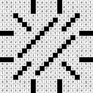
Figure 22.6 Solution for instance words-21 \(\mathtt{\times}\) 21-10

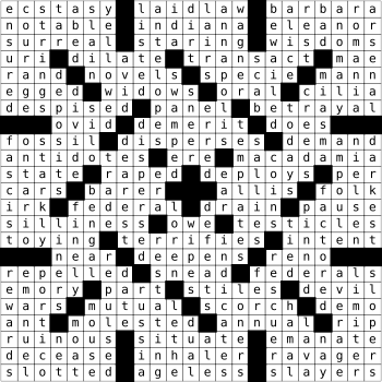
Figure 22.7 Solution for instance words-23 \(\mathtt{\times}\) 23-06

A solution for words-21 \(\mathtt{\times}\) 21-10 is shown in Figure 22.6 . A solution for words-23 \(\mathtt{\times}\) 23-06 is shown in Figure 22.7 . Note that words-23 \(\mathtt{\times}\) 23-10 does in fact not have a solution.

22.4.6. Acknowledgments.

We are grateful to Peter Van Beek for access to example grids and to Adi Botea for providing us with the dictionaries words and uk from [1] .