4. Integer and Boolean variables and constraints

This chapter gives an overview of integer and Boolean variables and the constraints available for them in Gecode. The chapter focuses on variables and constraints, a discussion of branching for integer and Boolean variables can be found in Branching on integer and Boolean variables.

The chapter does not make an attempt to duplicate the reference documentation (see Using integer variables and constraints). It is concerned with the most important ideas and principles underlying integer and Boolean variables and constraints. In particular, the chapter provides entry points into the reference documentation and points to illustrating examples.

Overview. Integer and Boolean variables details how integer and Boolean variables (and variables in general) can be used for modeling. Variable arrays and argument arrays are discussed in Variable and argument arrays. Important aspects of how constraints are posted in Gecode are explained in Posting constraints. These sections belong to the basic reading material of Modeling.

The remaining sections Constraint overview and Synchronized execution provide an overview of the constraints that are available for integer and Boolean variables in Gecode.

Important

Do not forget to add

#include <gecode/int.hh>

to your program when you want to use integer or Boolean variables and constraints.

All program fragments and references to classes, namespaces, and other entities assume that declarations and definitions from the Gecode namespace are visible: for example, by adding

using namespace Gecode;

to your program.

The variable home refers to a space reference (of type Space&) and defines the home space in which new variables, propagators, and branchers are posted. Often (as in Getting started and Getting comfortable) home will be *this, referring to the current space.

4.1. Integer and Boolean variables

Variables in Gecode are for modeling. They provide operations for creation, access, and update during cloning. By design, the only way to modify (constrain) a variable is by post functions for constraints and branchers.

Integer variables are instances of the class IntVar while Boolean variables are instances of the class BoolVar. Integer variables are not related to Boolean variables. A Boolean variable is not an integer variable with a domain that is included in \(\{0,1\}\). The only way to get an integer variable that is equal to a Boolean variable is by posting a channeling constraint between them (see Channel constraints).

Tip 4.1 (Do not use views for modeling).

If you — after some browsing of the reference documentation — should come across integer views such as IntView, you might notice that views have a richer interface than integer variables. You might feel that this interface looks too powerful to be ignored. Now, you really should put some trust in this document: views are not for modeling.

The more powerful interface only works within propagators and branchers, see Programming propagators and Programming branchers.

◄

4.1.1. Creating integer variables

A variable provides a read-only interface to a variable implementation where the same variable implementation can be referred to by arbitrarily many variables.

New integer variables are created by using a constructor. A new integer variable x is created by

IntVar x(home, -4, 20);

This declares a variable x of type IntVar in the space home, creates a new integer variable implementation with domain \(\{-4,\ldots,20\}\), and points x to the newly created integer variable implementation.

The domain of a variable can also be specified by an integer set IntSet, for example by

IntVar x(home, IntSet(-4, 20));

which creates a new variable with domain \(\{-4,\ldots,20\}\). An attempt to create an integer variable with an empty domain throws an exception of type Int::VariableEmptyDomain.

Integer sets can be initialized by an array of integers, for example

int v[] = {1,2,3,4};
IntSet c(v, 4);

initializes c to have the four elements (as defined by the second argument 4 in the constructor call) \(\{\mathtt{1},\mathtt{2},\mathtt{3},\mathtt{4}\}\), whereas

int r[][2] = {{1,2},{5,7}};
IntSet d(r, 2);

initializes d to have the elements \(\{\mathtt{1},\mathtt{2},\mathtt{5},\mathtt{6},\mathtt{7}\}\) where r is an array of pairs expressing ranges of values. The same can be expressed with initializer lists as in

IntSet c({1,2,3,4});
IntSet d({{1,2},{5,7}});

Please note the difference between IntSet({1,3}) and IntSet(1,3): the former has the elements \(\{\mathtt{1},\mathtt{3}\}\). while the latter has the elements \(\{\mathtt{1},\mathtt{2},\mathtt{3}\}\).

The default or copy constructor of a variable does not create a new variable (that is, a new variable implementation). Instead, the variable does not refer to any variable implementation (default constructor) or to the same variable implementation (copy constructor). For example, in

IntVar x(home, 1, 4);
IntVar y(x);

both x and y refer to the same integer variable implementation. Using a default constructor and an assignment operator is equivalent:

IntVar x(home, 1, 4);
IntVar y;
y=x;

4.1.2. Limits for integer values

The set of values for an integer variable is a subset of the values of the type int. The set of values is symmetric: \(-\mbox{\texttt{Int::Limits::min}}=\mbox{\texttt{Int::Limits::max}}\) for the smallest possible integer variable value Int::Limits::min and the largest possible integer variable value Int::Limits::max. Moreover, Int::Limits::max is strictly smaller than the largest possible integer value INT_MAX and Int::Limits::min is strictly larger than the smallest possible integer value INT_MIN. These limits are defined in the namespace Int::Limits.

Any attempt to create a variable with values outside the defined limits throws an exception of type Int::OutOfLimits. The same holds true for any attempt to use an integer value outside the defined limits when posting a constraint or brancher.

4.1.3. Variable domains are never empty

An important invariant in Gecode is that the domain of a variable is never empty. When a variable domain should become empty during propagation, the space is failed but the variable’s domain is kept. In fact, this is the very reason why an attempt to create a variable with an empty domain, for example by

IntVar x(home, 1, 0);

throws an exception of type Int::VariableEmptyDomain.

Tip 4.2 (Small variable domains are beautiful).

It is not an omission that an integer variable has no constructor that creates a variable with the largest possible domain. One could argue that a constructor like that would come in handy for creating temporary variables. After all, one would not have to worry about the exact domain!

Sorry, but one has to worry. The apparent omission is deliberate to make you worry indeed. For many propagators posted for a constraint a small domain is essential. For example, when posting a linear constraint (as in A first Gecode model), variable domains that are too large might result in an exception of type Int::OutOfLimits as during propagation numerical overflow might occur (even if Gecode resorts to a number type supporting larger numbers than int for propagating linear). Moreover, the runtime of other propagators (for example, many domain propagators such as domain consistent distinct) depend critically on the size of a domain. Again, Gecode tries to be clever in most of the cases. But, it is better to make it a habit to think about initial variable domains carefully (please remember: better safe than sorry).

For examples where small variable domains matter, see Small variable domains are still beautiful and Small variable domains are still beautiful.

◄

4.1.4. Creating Boolean variables

The only difference between integer and Boolean variables is that Boolean variables can only take the values 0 or 1. Any attempt to create a Boolean variable with values different from 0 or 1 throws an exception of type Int::NotZeroOne.

If Boolean variables are not explicitly mentioned in the following, the same functionality for integer variables is also available for Boolean variables and has the same behavior.

4.1.5. Variable access functions

Variables provide member functions for access, such as x.min() for the minimum value of the current domain for an integer or Boolean variable x. In particular, the member function x.val() accesses the integer value of an already assigned variable (if the variable is not yet assigned, an exception of type Int::ValOfUnassignedVar is thrown). In addition, variables can be printed by the standard output operator <<.

4.1.6. Iterating over integer variable domains

The entire domain of an integer variable can be accessed by a value iterator IntVarValues or a range iterator IntVarRanges. For example, the loop

for (IntVarValues i(x); i(); ++i)
  std::cout << i.val() << ' ';

uses the value iterator i to print all values of the domain of the integer variable x. The call operator i() tests whether there are more values to iterate for i, the prefix increment operator ++i moves the iterator i to the next value, and i.val() returns the current value of the iterator i. The values are iterated in strictly increasing order.

Similarly, the following loop

for (IntVarRanges i(x); i(); ++i)
  std::cout << i.min() << ".." << i.max() << ' ';

uses the range iterator i to print all ranges of the integer variable x. Given a finite set of integers \(d\), the range sequence of \(d\) is the shortest (and unique) sequence of ranges (intervals)

\[\langle\left[n_0..m_0\right]\},\ldots,\left[n_k..m_k\right]\}\rangle \]

such that the sequence is ordered and non-adjacent (\(m_i+1<n_{i+1}\) for \(0\leq i<k\)). A range iterator iterates over the ranges in the range sequence of a variable’s domain. Like a value iterator, a range iterator implements the call operator i() to test whether there are more ranges to iterate for i and the prefix increment operator ++i to move i to the next range. As a range iterator i iterates over ranges, it implements the member functions i.min() and i.max() for the minimal, respectively maximal, value of the current range.

Iteration of values and ranges for Boolean variables is not available (as it is not needed).

4.1.7. When to inspect a variable

Note that one must not change the domain of a variable (for example, by posting a constraint on that variable) while an iterator for that variable is still in use. This is the same as for most iterators, for example, for iterators in the C++ Standard Template Library (STL).

Otherwise, a variable can always be inspected: at any place (that is, not only in member functions of the variable’s home) and at any time (regardless of the status of a space). If the variable’s home is failed, the variable can still be inspected. However, it might be the case that the variable domain has more values than expected. For example, after creating a variable x with the singleton domain \(\{0\}\) and posting the constraint that x must be different from 0 by (read Propagation is explicit about status()):

IntVar x(home, 0, 0);
rel(home, x, IRT_NQ, 0);
(void) home.status();

the space home is failed but the variable x still contains the value 0 in its domain.

4.1.8. Updating variables

As discussed in A first Gecode model, a variable must be updated during cloning in the copy constructor used by a space’s copy() member function. For example, a variable x is updated by

x.update(home, y);

where y is the variable from which x is to be updated. While x belongs to home, y belongs to the space being cloned.

A space only needs to update the variables that are part of the solution, so that their values can be accessed after a solution space has been found. Temporary variables do not need to be copied.

Assume that we want to constrain the integer variable p to be the product of x, y, and z. Gecode only offers multiplication of two variables, hence a temporary variable t is created (assume also that we know that the values for t are between 0 and 1000):

IntVar t(home, 0, 1000);
mult(home, x, y, t);
mult(home, t, z, p);

Here, t does not require updating. The multiplication propagators created by mult take care of updating the variable implementation of t.

4.2. Variable and argument arrays

Gecode has very few proper data structures. The proper data structures for integer and Boolean variables are the variables themselves, integer sets, and arrays of variables. Proper means that these data structures can be updated and hence be stored in a space.

Of course, data structures that themselves do not contain proper data structures can be stored in a space, such as integers, pointers, and strings.

Gecode supports the programming of new proper data structures, this is discussed in Shared objects and handles.

4.2.1. Integer and Boolean variable arrays

Integer variable arrays of type IntVarArray can be used like variables. For example,

IntVarArray x(home, 4, -10, 10);

creates a new integer variable array with four variables containing newly created variables with domain \(\{-10,\ldots,10\}\). Boolean variable arrays of type BoolVarArray are analogous.

Creation of a variable array allocates memory from the home space. The memory is freed when the space is deleted (not when the destructor of the variable array is called). Variable arrays can be created without creating new variables by just passing the size. That is,

IntVarArray x(home, 4);
for (int i=0; i<4; i++)
  x[i] = IntVar(home, -10, 10);

is equivalent to the previous example.

The other operations on variable arrays are as one would expect. For example, one can check whether all variables are assigned using the assigned() function. More importantly, variable arrays like variables have an update function and variable arrays must be updated during cloning. In the following, we will refer to the size of a variable array x by \(|\mathtt x|\) (which can be computed by x.size()).

Matrix interface. Many models are naturally expressed by using matrices. Gecode offers support that superimposes a matrix interface for modeling on an array, see Matrix interface for arrays.

4.2.2. Argument arrays

As mentioned above, the memory allocated for a variable array is freed only when its home space is deleted. That makes variable arrays unsuited for temporary variable arrays, in particular for arrays that are built dynamically or used as arguments for post functions.

For this reason, Gecode provides argument arrays: IntVarArgs for integer variables, BoolVarArgs for Boolean variables, IntArgs for integers, and IntSetArgs for integer sets (see Argument arrays). Internally, they allocate space from the heap [1] and the memory is freed when their destructor is executed.

Argument arrays can be created empty:

IntVarArgs x;

with a certain size but without initializing the elements:

IntVarArgs x(5);

using standard initializer lists (assuming that a, b, c, and d are integer variables):

IntVarArgs x({a,b,c,d});

or fully initialized:

IntVarArgs x(home,5,0,10);

For a typical example, consider A first Gecode model where an integer argument array and an integer variable argument array are used to pass coefficients and variables to the linear post function.

Dynamic argument arrays. In contrast to variable arrays, argument arrays can grow dynamically by adding elements or whole arrays using operator<<:

IntVarArgs x;
x << IntVar(home,0,10);
IntVarArgs y;
y << IntVar(home,10,20);
y << x;
linear(home, IntVarArgs()<<x[0]<<x[1], IRT_EQ, 0);

Furthermore, argument arrays can be concatenated using operator+:

IntVarArgs z = x+y;

Slices. It is sometimes necessary to post constraints on a subsequence of the variables in an array. This is made possible by the slice(start,inc,n) method of variable and argument arrays. The start parameter gives the starting index of the subsequence. The inc optional parameter gives the increment, i.e., how to get from one element to the next (its default is \(1\)). The n parameter gives the maximal length of the resulting array (its default is \(-1\), meaning as long as possible).

The following examples should make this clearer. Assume that the integer variable argument array x is initialized as follows:

IntVarArgs x(home, 10, 0, 10);

Then the following calls of slice() return:

• x.slice(5) returns an array with elements x[5],x[6],…,x[9].

• x.slice(5,1,3) returns x[5],x[6],x[7].

• x.slice(5,-1) returns x[5],x[4],…,x[0].

• x.slice(3,3) returns x[3],x[6],x[9].

• x.slice(8,-2) returns x[8],x[6],x[4],x[2],x[0].

• x.slice(8,-2,3) returns x[8],x[6],x[4].

Tip 4.3 (Reversing argument arrays).

The slice() method can be used to compute an array with the elements of x in reverse order like this:

x.slice(x.size()-1,-1)

◄

Creating integer argument arrays. Integer argument arrays support standard initializer lists, for example

IntArgs c({0,1,2,3});

creates an array with the four elements 0, 1, 2, and 3.

Integer argument arrays with simple sequences of integers can be generated using the static method IntArgs::create(n,start,inc). The n parameter gives the length of the generated array. The start parameter is the starting value, and inc determines the increment from one value to the next.

Here are a few examples:

• IntArgs::create(5,0) creates an array with elements 0,1,2,3,4.

• IntArgs::create(5,4,-1) creates 4,3,2,1,0.

• IntArgs::create(3,2,0) creates 2,2,2.

• IntArgs::create(6,2,2) creates 2,4,6,8,10,12.

Tip 4.4 (Dynamically constructing models).

Sometimes the number of variables cannot be determined easily, for example when it depends on data read from a file.

Suppose the following script with a variable array x:

dynamic script ≡

  class Script : public Space {
    IntVarArray x;
  public:
    // [dynamic script:read data]
      // [dynamic script:initialize variable array]
    }
    ...
  }

It is easy to use a variable argument array _x for collecting variables as follows:

read data ≡

      IntVarArgs _x;
      while (...) {
        ...
        _x << IntVar(*this,...);
      }

and then initialize the variable array x using the argument array:

initialize variable array ≡

      x = IntVarArray(*this,_x);

◄

In the following we do not distinguish between arrays and argument arrays unless operations require a certain type of array. In fact, all post functions for constraints and branchers only accept variable argument arrays. A variable array is automatically casted to a variable argument array if needed.

4.2.3. STL-style iterators

All arrays in Gecode (including variable arrays and argument arrays) also support STL-style (Standard Template Library) iterators. For example, assume that a is an integer variable argument array. Then

for (IntVarArgs::iterator i = a.begin(); i != a.end(); ++i) {
   ...
}

creates an iterator i for the elements of a and iterates from the first to the last element in a.

More powerfully, iterators give you the ability to work with STL algorithms. Suppose that f() is a function that takes an integer variable by reference such as in

void f(IntVar& x) { ... }

and a is an integer variable argument array. Then

#include <algorithm>

std::for_each(a.begin(), a.end(), f); 

applies the function f() to each integer variable in a.

4.3. Posting constraints

This section provides information about general principles for posting constraints over integer and Boolean variables.

4.3.1. Post functions are clever

A constraint post function carefully analyzes its arguments. Based on this analysis, the constraint post function chooses the best possible propagator for the constraint.

For example, when posting a distinct constraint (see Distinct constraints) for the variable array x by

distinct(home, x);

where x has two elements, the much more efficient propagator for disequality \(\mathtt{x}_0 \neq \mathtt{x}_1\) is created.

4.3.2. Everything is copied

When passing arguments to a post function, all data structures that are needed for creating a propagator (or several propagators) implementing a constraint are copied. That is, none of the data structures that are passed as arguments are needed after a constraint has been posted.

4.3.3. Reified constraints

Many constraints also exist as reified variants: the validity of a constraint is reflected to a Boolean control variable (reified constraints are also known as meta-constraints). In addition to full reification also half reification [15] is supported for reified constraints. Whether a reified version exists for a given constraint can be found in the reference documentation. If a reified version does exist, the Boolean control variable (and possibly information about the reification mode, to be discussed in Half reification) is passed as the last non-optional argument.

For example, posting

rel(home, x, IRT_EQ, y, b);

for integer variables x and y and a Boolean control variable b creates a propagator for the reified constraint \(\reifyeqv{\mathtt{b}}{\mathtt{x}=\mathtt{y}}\) that propagates according to the following rules:

• If b is assigned to 1, the constraint \(\mathtt{x}=\mathtt{y}\) is propagated.

• If b is assigned to 0, the constraint \(\mathtt{x}\neq\mathtt{y}\) is propagated.

• If the constraint \(\mathtt{x}=\mathtt{y}\) holds, then \(\mathtt{b}=\mathtt{1}\) is propagated.

• If the constraint \(\mathtt{x}\neq\mathtt{y}\) holds, then \(\mathtt{b}=\mathtt{0}\) is propagated.

4.3.4. Half reification

Reification as discussed in the previous paragraph is also known as full reification as it propagates a full equivalence between the constraint \(c\) and the constraint that a Boolean control variable is equal to 1. Half reification propagates only one direction of the equivalence [15]. Half reification can be used by passing an object of class Reify that combines a Boolean control variable and a reification mode of type ReifyMode (see Using integer variables and constraints).

For example, the half reified constraint \(\reifyimp{\mathtt{b}}{\mathtt{x}=\mathtt{y}}\) for integer variables x and y and a Boolean control variable b can be posted by

Reify r(b, RM_IMP);
rel(home, x, IRT_EQ, y, r);

and is propagated as follows (RM_IMP suggests implication \(\Rightarrow\)):

• If b is assigned to 1, the constraint \(\mathtt{x}=\mathtt{y}\) is propagated.

• If the constraint \(\mathtt{x}\neq\mathtt{y}\) holds, then \(\mathtt{b}=\mathtt{0}\) is propagated.

Likewise, the half reified constraint \(\reifypmi{\mathtt{b}}{\mathtt{x}=\mathtt{y}}\) for integer variables x and y and a Boolean control variable b can be posted by

Reify r(b, RM_PMI);
rel(home, x, IRT_EQ, y, r);

and is propagated as follows (RM_PMI suggests inverse implication \(\Leftarrow\)):

• If b is assigned to 0, the constraint \(\mathtt{x}\neq\mathtt{y}\) is propagated.

• If the constraint \(\mathtt{x}=\mathtt{y}\) holds, then \(\mathtt{b}=\mathtt{1}\) is propagated.

Full reification can be requested by the reification mode RM_EQV (for equivalence \(\Leftrightarrow\)) as follows:

Reify r(b, RM_EQV);
rel(home, x, IRT_EQ, y, r);

As the constructor for Reify has RM_EQV as default value for its second argument, this can be written shorter as:

Reify r(b);
rel(home, x, IRT_EQ, y, r);

or even shorter as:

rel(home, x, IRT_EQ, y, b);

For convenience, three functions eqv(), imp(), and pmi() exist that take a Boolean variable and return a corresponding object of class Reify. For example, instead of writing:

Reify r(b, RM_IMP);
rel(home, x, IRT_EQ, y, r);

one can write more concisely:

rel(home, x, IRT_EQ, y, imp(b));

4.3.5. Selecting the propagation level

For many constraints, Gecode provides different propagators with different levels of propagation. All constraint post functions take an optional argument of type IntPropLevel (see Using integer variables and constraints) controlling which propagator is chosen for a particular constraint.

The different simple values for IntPropLevel have the following meaning:

• IPL_VAL: perform value propagation. A typical example is naive distinct: wait until a variable becomes assigned to a value \(n\), then prune \(n\) from all other variables.

• IPL_BND: perform bounds propagation or achieve bounds consistency. This captures both bounds consistency over the integers (for example, for distinct, see Distinct constraints) or bounds consistency over the real numbers (for example, for linear, see Linear constraints). For more information on bounds consistency over integers or real numbers, see [11].

  Some propagators that are selected might not even achieve bounds consistency but the idea is that the propagator performs propagation by reasoning on the bounds of variable domains.

• IPL_DOM: perform domain propagation or achieve domain consistency. Most propagators selected by IPL_DOM achieve domain consistency but some just perform propagation by taking entire variable domains for propagation into account (for example, circuit, see Circuit and Hamiltonian path constraints).

• IPL_DEF: choose default propagation level for this constraint.

Whether bounds or domain consistency is achieved and the default propagation level for a constraint are mentioned in the reference documentation for each post function.

In addition to the basic propagation levels listed above, the following pre-defined values exist:

• IPL_BASIC: try to optimize for execution performance at the expense of performing less propagation.

• IPL_ADVANCED: try to optimize for more propagation at the expensive of being less efficient.

The propagation levels can be specified as disjunctions, for example IPL_DEF|IPL_BASIC requests basic default propagation which is equivalent to IPL_BASIC (the IPL_DEF can always be omitted). Note that in particular the combination IPL_BASIC|IPL_ADVANCED is meaningful requesting both basic and advanced propagation to be performed.

Some scheduling constraints, see Scheduling constraints, support basic and advanced propagation levels.

Tip 4.5 (Different propagation levels have different costs).

Note that propagators of different propagation level for the very same constraint can have vastly different cost. In general, propagation for IPL_VAL will be cheapest, while propagation for IPL_DOM will be most expensive.

The reference documentation for a constraint lists whether a particular propagation level might have prohibitive cost for a large number of variables or a large number of values in the variables’ domains. For example, for the linear constraint with \(n\) variables and at most \(d\) values for each variable, the complexity to perform bounds propagation (that is, IPL_BND) is \(O(n)\) whereas the complexity for domain propagation (that is, IPL_DOM) is \(O(d^n)\).

◄

4.3.6. Exceptions

Many post functions check their arguments for consistency before attempting to create a propagator. For each post function, the reference documentation lists which exceptions might be thrown.

4.3.7. Unsharing arguments

Some constraints can only deal with non-shared variable arrays: a variable is not allowed to appear more than once in the array (more precisely: no unassigned variable implementation appears more than once in the array). An attempt to post one of these constraints with shared variable arrays will throw an exception of type Int::ArgumentSame.

To be able to post one of these constraints on shared variable arrays, Gecode provides a function unshare (see Unsharing variables) that takes a variable argument array x as argument as in:

unshare(home, x);

It replaces each but the first occurrence of a variable \(y\) in x by a new variable \(z\), and creates a propagator \(y=z\) for each new variable \(z\).

Note that unshare requires a variable argument array and not a variable array. If x is a variable array, the following

IntVarArgs y(x);

creates a variable argument array y containing the same variables as x.

Tip 4.6 (Unsharing is expensive).

It is important to keep in mind that unshare creates new variables and propagators. This is also the reason why unsharing is not done implicitly by a post function for a constraint that does not accept shared variable arrays.

Consider the following example using extensional constraints for a variable argument array x possibly containing a variable more than once, where a and b are two different DFAs (see Extensional constraints for extensional constraints). By

unshare(home, x);
extensional(home, x, a);
extensional(home, x, b);

multiple occurrences of the same variable in x are unshared once and the propagators for extensional can work on the same non-shared array.

If unsharing were implicit, the following

extensional(home, x, a);
extensional(home, x, b);

would unshare x twice and create many more (useless) propagators and variables. Rather than implicitly unsharing the same array over and over again (and hence creating variables and propagators), unsharing is made explicit and should be done only once, if possible.

◄

4.4. Constraint overview

This section provides an overview of the constraints and their post functions available for integer and Boolean variables.

4.4.1. Domain constraints

Domain constraints constrain integer variables and variable arrays to values from a given domain. For example, by

dom(home, x, 2, 12);

the values of the variable x (or of all variables in a variable array x) are constrained to be between \(2\) and \(12\). Domain constraints also take integers (assigning variables to the integer value) and integer sets of type IntSet. For example,

IntArgs a({1,-3,5,-7})
IntSet d(a);
dom(home, x, d);

constrains the variable x (or, the variables in x) to take values from the set \(\{-7,-3,1,5\}\) (see also GCCat: domain, in, in_interval, in_intervals, in_set).

Note that there are no domain constraints for Boolean variables, please use relation constraints instead, see Simple relation constraints over Boolean variables.

The domain of an integer or Boolean variable x can be constrained according to the domain of another variable d by

dom(home, x, d);

Here, x and d can also be arrays of integer or Boolean variables. Note that this needs to be used carefully, the domain to which the variable x is constrained depends on the domain to which d is constrained. Only use this constraint post function if you are sure that all propagation that could influence the domain of d has been performed!

Domain constraints for a single variable also support reification. For examples using domain constraints, see n-Knight’s tour (simple model) and Packing squares into a rectangle.

4.4.2. Membership constraints

Membership constraints constrain integer or Boolean variables to be included in an array of integer or Boolean variables. That is, for an integer variable array x and an integer variable y, the constraint

member(home, x, y);

forces that y is included in x:

\[\mathtt{y}\in\left\{\mathtt{x}_0,\ldots,\mathtt{x}_{|\mathtt{x}|-1}\right\} \]

As mentioned, x and y can also be Boolean variables. Membership constraints also support reification.

4.4.3. Simple relation constraints over integer variables

IRT_EQ	equality (\(=\))	IRT_NQ	disequality (\(\neq\))
IRT_LE	strictly less inequality (\(<\))	IRT_LQ	less or equal inequality (\(\leq\))
IRT_GR	strictly greater inequality (\(>\))	IRT_GQ	greater or equal inequality (\(\geq\))

Figure 4.1 Integer relation types

Simple relation constraints over integer variables enforce relations between integer variables and between integer variables and integer values. The relation depends on an integer relation type IntRelType (see Simple relation constraints over integer variables). Figure 4.1 lists the available integer relation types and their meaning.

Binary relation constraints. Assume that x and y are integer variables. Then

rel(home, x, IRT_LE, y);

constrains x to be strictly less than y. Similarly, by

rel(home, x, IRT_NQ, 4);

x is constrained to be different from 4. Both variants of rel also support reification (see also GCCat: eq, neq, lt, leq, gt, geq).

Constraints between variable arrays and a single variable. If x is an integer variable array and y is an integer variable, then

rel(home, x, IRT_LQ, y);

constrains all variables in x to be less than or equal to y. Likewise,

rel(home, x, IRT_GR, 7);

constrains all variables in x to be larger than 7 (see also GCCat: arith).

Constraints between array elements. If x is an integer variable array, then

rel(home, x, IRT_LQ);

constrains the variables in x to be sorted in increasing order as follows:

\[\mathtt{x}_0 \leq \mathtt{x}_1 \leq \cdots \leq \mathtt{x}_{|\mathtt x|-1}\]

The integer relation type values for inequalities (that is, IRT_LE, IRT_GQ, and IRT_GR) are analogous. For an example, see Golomb rulers and Finding optimal Golomb rulers.

By

rel(home, x, IRT_EQ);

all variables in the integer variable array x are constrained to be equal:

\[\mathtt{x}_0 = \mathtt{x}_1 = \cdots = \mathtt{x}_{|\mathtt x|-1}\]

By

rel(home, x, IRT_NQ);

the variables in x are constrained to be not all equal:

\[\neg\left(\mathtt{x}_0 = \mathtt{x}_1 = \cdots = \mathtt{x}_{|\mathtt x|-1}\right)\]

For an example, see Schur’s lemma (see also GCCat: all_equal, decreasing, increasing, not_all_equal, strictly_decreasing, strictly_increasing).

Lexicographic constraints between variable arrays.

If x and y are integer variable arrays (where the sizes of x and y can be different),

rel(home, x, IRT_LE, y);

constrains x and y such that x is lexicographically strictly smaller than y (analogously for the other inequality relations). For IRT_EQ and \(|\mathtt x|=|\mathtt y|\), it is propagated that \(\mathtt x_i=\mathtt y_i\) for \(0\leq i<|\mathtt x|\). For IRT_NQ and \(|\mathtt x|=|\mathtt y|\), it is propagated that \(\mathtt x_i\neq \mathtt y_i\) for at least one \(i\) such that \(0\leq i<|\mathtt x|\). If \(|\mathtt x|\neq|\mathtt y|\), for IRT_EQ the space home is failed whereas for IRT_NQ the constraint is ignored (see also GCCat: lex_greater, lex_greatereq, lex_less, lex_lesseq).

See Balanced incomplete block design (BIBD) for an example (albeit over Boolean variables).

4.4.4. Simple relation constraints over Boolean variables

BOT_AND	conjunction (\(\wedge\))	BOT_OR	disjunction (\(\vee\))
BOT_IMP	implication (\(\rightarrow\))	BOT_EQV	equivalence (\(\leftrightarrow\))
BOT_XOR	exclusive or (\(\nleftrightarrow\))

Figure 4.2 Boolean operation types

Simple relation constraints over Boolean variables include the same post functions as simple relation constraints over integer variables. In addition, simple relation constraints over Boolean constraints provide support for the typical Boolean operations such as conjunction and disjunction. Boolean operations are defined by values of the type BoolOpType (see Simple relation constraints over integer variables). Figure 4.2 lists the available Boolean operation types.

For example, for Boolean variables x, y, and z,

rel(home, x, BOT_AND, y, z);

posts the constraint \(\mathtt{x}\wedge\mathtt{y}=\mathtt{z}\). Similarly,

rel(home, x, BOT_OR, y, 1);

posts that \(\mathtt{x}\vee\mathtt{y}\) must be true (see also GCCat: and, equivalent, imply, or, xor).

Note that the integer value must be either zero or one, otherwise an exception of type Int::NotZeroOne is thrown.

For an example, see Balanced incomplete block design (BIBD).

Tip 4.7 (Boolean negation).

Boolean negation can be easily obtained by using IRT_NQ as relation type. The constraint \(\mathtt{x}=\neg\mathtt{y}\) for Boolean variables x and y can be posted by

rel(home, x, IRT_NQ, y);

◄

Additional constraints are available for Boolean variable arrays. For a Boolean variable array x and a Boolean variable y,

rel(home, BOT_OR, x, y)

posts the constraint

\[\bigvee_{i=0}^{|\mathtt x|-1}\mathtt{x}_i=\mathtt{y} \]

Again, y can also be 0 or 1.

Note that Boolean implication is special in that it is not associative and Gecode follows normal notational convention. Hence for a Boolean variable array x and a Boolean variable y,

rel(home, BOT_IMP, x, y)

posts the constraint

\[\mathtt{x}_0 \to \left(\mathtt{x}_1 \to \left(\ldots\to\left(\mathtt{x}_{|\mathtt{x}|-2}\to \mathtt{x}_{|\mathtt{x}|-1}\right)\right)\right)=\mathtt{y}\]

Again, y can also be 0 or 1.

Clause constraint.

In order to avoid many propagators for negation, the clause constraint accepts both positive and negative Boolean variables. For Boolean variable arrays x and y and a Boolean variable z (again, z can also be 0 or 1)

clause(home, BOT_AND, x, y, z);

posts the constraint

\[\bigwedge_{i=0}^{|\mathtt{x}|-1}\mathtt{x}_i\wedge \bigwedge_{i=0}^{|\mathtt{y}|-1}\neg\mathtt{y}_i=\mathtt z\]

(see also GCCat: clause_and, clause_or, nand, nor).

Note that only BOT_AND and BOT_OR as Boolean operation types are supported, other Boolean operations types throw an exception of type Int::IllegalOperation.

For an example, see CNF SAT solver.

If-then-else constraint. An if-then-else constraint can be posted by

ite(home, b, x, y, z);

where b is a Boolean variable and x, y, and z are integer or Boolean variables. In case b is one, then \(\mathtt{x}=\mathtt{z}\) must hold, otherwise \(\mathtt{y}=\mathtt{z}\) must hold.

4.4.5. Arithmetic constraints

post function	constraint posted	bnd	dom	GCCat
min(home, x, y, z);	\(\min(\mathtt x, \mathtt y)=\mathtt z\)	yes	yes	minimum
max(home, x, y, z);	\(\max(\mathtt x, \mathtt y)=\mathtt z\)	yes	yes	maximum
abs(home, x, y);	\(|\mathtt x|=\mathtt y\)	yes	yes	abs_value
mult(home, x, y, z);	\(\mathtt x \cdot \mathtt y=\mathtt z\)	yes	yes
sqr(home, x, y);	\({\mathtt x}^2=\mathtt y\)	yes	yes
sqrt(home, x, y);	\(\lfloor\sqrt{\mathtt x}\rfloor=\mathtt y\)	yes	yes
pow(home, x, n, y);	\({\mathtt x}^{\mathtt n}=\mathtt y\)	yes	yes
nroot(home, x, n, y);	\(\lfloor\sqrt[{\mathtt n}]{\mathtt x}\rfloor=\mathtt y\)	yes	yes
div(home, x, y, z);	\(\mathtt{x} \div \mathtt{y}=\mathtt{z}\)	yes
mod(home, x, y, z);	\(\mathtt{x} \bmod \mathtt{y}=\mathtt{z}\)	yes
divmod(home, x, y, d, m);	\(\mathtt{x} \div \mathtt{y}=\mathtt{d}\wedge\mathtt{x} \bmod \mathtt{y}=\mathtt{m}\)	yes

Figure 4.3 Arithmetic constraints (x, y, z, d, and m are integer variables; n is an integer)

Arithmetic constraints exist only over integer variables. In addition to the constraints summarized in Figure 4.3 (bnd abbreviates bounds consistency and dom abbreviates domain consistency), the minimum and maximum constraints are also available for integer variable arrays. That is, for an integer variable array x and an integer variable y

min(home, x, y);

constrains y to be the minimum of the variables in x (max is analogous) (see also GCCat: min, max).

Also constraints for the arguments of minimum and maximum are available. For an integer variable array x and an integer variable y

argmin(home, x, y);

constrains y to be \(\argmin(\mathtt{x})\), that is, the element in x at position y is equal to \(\min(\mathtt{x})\) (see also GCCat: min_index). By default, argmin uses tie-breaking and constrains y to be the first position of the minimum in x. By posting

argmin(home, x, y, false);

no tie-breaking is used. Of course, argmax is analogous. argmin and argmax without tie-breaking are domain consistent (see also GCCat: max_index).

4.4.6. Linear constraints

Linear constraints over integer variables and Linear constraints over Boolean variables provide essentially the same post functions for integer and Boolean constraints (to be discussed below). The most general variant

linear(home, a, x, IRT_EQ, c);

posts the linear constraint

\[\sum_{i=0}^{|\mathtt x|-1} \mathtt{a}_i \cdot \mathtt{x}_i = \mathtt c\]

with integer coefficients a (of type IntArgs), integer variables x, and an integer constant c. Note that a and x must have the same size. Of course, all other integer relation types are supported, see Figure 4.1 for a table of integer relation types. Multiple occurrences of the same variable in x are explicitly allowed and common terms \(a\cdot y\) and \(b\cdot y\) for the same variable \(y\) are rewritten to \((a+b)\cdot y\) to increase propagation. For an example, see A first Gecode model.

The array of coefficients can be omitted if all coefficients are one. That is,

linear(home, x, IRT_GR, c);

posts the linear constraint

\[\sum_{i=0}^{|\mathtt x|-1} \mathtt{x}_i > \mathtt c \]

for a variable array x and an integer c.

Instead of an integer constant c as the right-hand side of the linear constraint, an integer variable can be used as well. This is true for linear constraints over both integer and Boolean variables: the right-hand side is always an integer value or an integer variable, even if the left-hand side involves Boolean variables. For example, when assuming that x is an array of Boolean variables,

linear(home, x, IRT_GQ, y);

imposes the constraint that there are at least y ones among the Boolean variables in x.

All variants of linear support reification and exist in variants that perform both bounds propagation (the default) and domain propagation (see also GCCat: scalar_product, sum_ctr).

4.4.7. Distinct constraints

The distinct constraint (see Distinct constraints) enforces that integer variables take pairwise distinct values (also known as alldifferent constraint). Obviously, distinct does not exist for Boolean variables.

Posting

distinct(home, x);

constrains all variables in x to be pairwise different.

Posting

distinct(home, c, x);

for an array of integer values c (of type IntArgs) and an array of integer variables x of same size, constrains the variables in x such that

\[\mathtt{x}_i+\mathtt{c}_i \neq\mathtt{x}_j+\mathtt{c}_j \qquad\mbox{for }0\leq i,j< |\mathtt{x}|\mbox{ and }i\neq j\]

Additionally, two variants of distinct are available where not all variables need to be pairwise different. Posting

distinct(home, x, c);

for an array of integer variables x and an integer value c constrains all variables in x to be different or equal to c:

\[\mathtt{x}_i=\mathtt{c}\vee\mathtt{x}_j=\mathtt{c}\vee\mathtt{x}_i \neq\mathtt{x}_j \qquad\mbox{for }0\leq i,j< |\mathtt{x}|\mbox{ and }i\neq j\]

For an array of Boolean variables b and an array of integer variables x of same size, posting

distinct(home, b, x);

constrains all variables in x to be different provided the respective Boolean variable is one:

\[\mathtt{b}_i=0\vee\mathtt{b}_j=0\vee\mathtt{x}_i \neq\mathtt{x}_j \qquad\mbox{for }0\leq i,j< |\mathtt{x}|\mbox{ and }i\neq j\]

Gecode offers value (the default), bounds (based on [32]), and domain propagation (based on [44]) for distinct (see also GCCat: alldifferent, alldifferent_cst, alldifferent_except_0).

For examples, see in particular Golomb rulers, n-Queens puzzle, and Crowded chessboard.

4.4.8. Counting constraints

Counting single values. Counting constraints count how often values are taken by an array of integer variables. The simplest case is

count(home, x, y, IRT_EQ, z);

which constrains z to be equal (controlled by IRT_EQ, all integer relation types are supported, see Figure 4.1) to the number of integer variables in x that are equal to y. Here y and z can be integer variables as well as integer values (see also GCCat: atleast, atmost, count, exactly).

The count constraints also support counting how many integer variables are included in an integer set. If y is an integer set, then

count(home, x, y, IRT_EQ, z);

constrains z to be equal to the number of integer variables in x that are included in y (see also GCCat: among, among_var, counts).

The following

count(home, x, c, IRT_EQ, z);

where x is an array of integer variables and c is an array of integers (of type IntArgs) with same size and z is an integer variable or value, constrains z to how often \(\mathtt{x}_i=\mathtt{c}_i\), that is

\[\mathtt{z}=\#\{i\in\{0,\ldots,|\mathtt{x}|-1\}\mid\mathtt{x}_i=\mathtt{c}_i\} \]

Here, \(\#s\) denotes the cardinality (number of elements) of a set \(s\).

Counting multiple values. The count constraint also supports counting multiple values (also known as gcc, or global cardinality constraint). Suppose that x and y (the counting variables) are two integer variable arrays (not necessarily of the same size). Then

count(home, x, y);

posts the constraints that the number of variables in x that are equal to a value \(j\) is \(\mathtt{y}_j\) (for \(0\leq j<|\mathtt y|\)):

\[\#\{i\in\{0,\ldots,|\mathtt{x}|-1\}\mid\mathtt{x}_i=j\}=\mathtt{y}_j \qquad\mbox{for }0\leq j<|\mathtt{y}|\]

and that no other values are taken by x:

\[\bigcup_{i=0}^{|\mathtt{x}|-1} \{\mathtt{x}_i\} = \{0,\ldots,|\mathtt y|-1\}\]

Rather than using counting variables, one can also use an array of integer sets (IntSetArgs). Then the number of values taken must be included in each individual set.

A more general variant also takes into account that the values under consideration are non contiguous but are defined by an additional array of integer values. Suppose that x and y (the counting variables) are two integer variable arrays (not necessarily of the same size) and c is an array of integers with the same size as y.

Then,

count(home, x, y, c);

posts the constraints that the number of variables in x that are equal to the value \(\mathtt{c}_j\) is \(\mathtt{y}_j\) (for \(0\leq j<|\mathtt y|\)):

\[\#\{i\in\{0,\ldots,|\mathtt{x}|-1\}\mid\mathtt{x}_i=\mathtt{c}_j\} =\mathtt{y}_j \qquad\mbox{for }0\leq j<|\mathtt{y}|\]

and that no other values but those in c are taken by x:

\[\bigcup_{i=0}^{|\mathtt{x}|-1} \{\mathtt{x}_i\} = \bigcup_{i=0}^{|\mathtt{c}|-1} \{\mathtt{c}_i\}\]

Again, y can also be an array of integer sets, where equality \(=\) is replaced by set inclusion \(\in\).

A slightly simpler variant replaces the cardinality variables by a single integer set. That is, for an array of integer variables x, an integer set d, and an array of integer values c

count(home, x, d, c);

posts the constraints that the number of variables in x that are equal to the value \(\mathtt{c}_j\) is included in \(\mathtt{d}\) (for \(0\leq j<|\mathtt c|\)):

\[\#\{i\in\{0,\ldots,|\mathtt{x}|-1\}\mid\mathtt{x}_i=\mathtt{c}_j\} \in\mathtt{d} \qquad\mbox{for }0\leq j<|\mathtt{c}|\]

and that no other values but those in c are taken by x:

\[\bigcup_{i=0}^{|\mathtt{x}|-1} \{\mathtt{x}_i\} = \bigcup_{i=0}^{|\mathtt{c}|-1} \{\mathtt{c}_i\}\]

The last variant of count clarifies that count is a generalization of distinct (see Distinct constraints): distinct constrains a value to occur at most once, whereas count offers more flexibility to constrain which values and how often these values can occur.

For example, if we know that the variables in the variable array x take values between 0 and n-1, then

count(home, x, IntSet(0,1), IntArgs::create(n,0,1));

is equivalent to

distinct(home, x);

Counting constraints only support integer variables, linear constraints can be used for Boolean variables, see Linear constraints. For examples, see the case studies in Magic sequence and Locating warehouses or the examples Crowded chessboard and Magic sequence.

Note that Gecode implements the semantics of the original paper on the global cardinality constraint by Régin [43], where no other values except those specified may occur. This differs from the semantics in the Global Constraint Catalog [6], where values that are not mentioned can occur arbitrarily often.

Gecode offers value (the default), bounds (based on [41]), and domain propagation (based on [43]) for the global count constraint (see also GCCat: global_cardinality).

4.4.9. Number of values constraints

Number of values constraints constrain how many values can be taken by an array of variables.

Assume that x is an array of integer variables and y is an integer variable. Then

nvalues(home, x, IRT_EQ, y);

constrains the number of distinct values in x to be equal to y, that is

\[\#\{\mathtt{x}_0,\ldots,\mathtt{x}_{|\mathtt{x}|-1}\}=\mathtt y \]

Instead of IRT_EQ any other integer relation type can be used, see Figure 4.1 for an overview. For example,

nvalues(home, x, IRT_LQ, y);

constrains the number of distinct values in x to be less than or equal to y. The array x can also be an array of Boolean variables and y can be an integer value.

The constraint is implemented by the propagators introduced in [7] (see also GCCat: nvalue, nvalues). For an example using the nvalues constraint, see Dominating Queens.

4.4.10. Sequence constraints

Sequence constraints constrain how often values are taken by repeated subsequences of variables in an array of integer or Boolean variables. By

sequence(home, x, s, q, l, u);

where x is an array of integer or Boolean variables, s is an integer set, and q, l, and u are integers, all subsequences of length q in the variable array x, that is, the sequences

\[\begin{array}{c} \langle \mathtt{x}_0,\ldots,\mathtt{x}_{\mathtt{q}+0-1} \rangle\\ \langle \mathtt{x}_1,\ldots,\mathtt{x}_{\mathtt{q}+1-1} \rangle\\ \cdots\\ \langle \mathtt{x}_{|\mathtt{x}|-\mathtt{q}},\ldots,\mathtt{x}_{|\mathtt{x}|-1} \rangle\\ \end{array}\]

are constrained such that at least l and at most u variables in each subsequence are assigned to values from the integer set s.

In more mathematical notation, the constraint enforces

\[\bigwedge_{i=0}^{|\mathtt{x}|-\mathtt{q}} \operatorname{among}(\langle \mathtt{x}_i,\ldots,\mathtt{x}_{i+\mathtt{q}-1}\rangle, \mathtt{s},\mathtt{l},\mathtt{u})\]

where the \(\operatorname{among}\) constraint for the subsequence starting at position \(i\) is defined as

\[l\leq\#\{j\in\{i,\ldots,i+\mathtt{q}-1\}\;|\;x_j\in \mathtt{s}\} \leq u \]

The constraint is implemented by the domain consistent propagator introduced in [62] (see also GCCat: among_seq). For an example, see Car sequencing.

4.4.11. Channel constraints

Channel constraints channel Boolean to integer variables and integer variables to integer variables.

Channeling integer variables. For two integer variable arrays x and y of same size,

channel(home, x, y);

posts the constraint

\[\mathtt{x}_i=j\iff\mathtt{y}_j=i \qquad\mbox{for }0\leq i,j<|\mathtt x|\]

(see also GCCat: inverse). The channel constraint between two integer variable arrays also supports integer offsets. For integers n and m,

channel(home, x, n, y, m);

posts the constraint

\[\mathtt{x}_i-\mathtt n=j\iff\mathtt{y}_j-\mathtt m=i \qquad\mbox{for }0\leq i,j<|\mathtt x|\]

(see also GCCat: inverse_offset). For examples, see n-Knight’s tour (simple model) and Black hole patience.

Channeling between integer and Boolean variables. As integer and Boolean variables are unrelated (see Integer and Boolean variables), the only way to express that a Boolean variable x is equal to an integer variable y is by posting either

channel(home, x, y);

or

channel(home, y, x);

The channel constraint can also map an integer variable y to an array of Boolean variables x. The constraint

\[\mathtt{x}_i=1 \iff \mathtt y = i\qquad\mbox{for }0\leq i<|x| \]

is posted by

channel(home, x, y);

(see also GCCat: domain_constraint). Note that an optional offset argument is supported. The constraint

\[\mathtt{x}_i=1 \iff \mathtt y = i+\mathtt n\qquad\mbox{for }0\leq i<|x| \]

for an integer value n is posted by

channel(home, x, y, n);

For an example, see Pentominoes.

4.4.12. Element constraints

Element constraints generalize array access to integer variables. For example,

IntArgs c({1,4,9,16,25});
element(home, c, x, y);

constrains the integer variable y to be the element of the array c at index x (where the array starts at index 0 as is common in C++).

The index variable x is always an integer variable, but the array c can also be an array of integer variables, Boolean variables, or an array of integers between 0 and 1. The result variable y must be a Boolean variable or an integer between 0 and 1 if the array is an array of Boolean variables. It can be a Boolean variable if all integer values in the array are between 0 and 1.

Even if bounds propagation is requested for the element constraint, the propagators for element always perform domain reasoning on the index variable (see also GCCat: elem, element). For examples, see the case study in Locating warehouses or the examples Steel-mill slab design problem and Travelling salesman problem (TSP).

Tip 4.8 (Shared integer arrays).

When checking the documentation for Element constraints it might come at a surprise that element constraints do not take integer argument arrays of type IntArgs but shared integer arrays of type IntSharedArray as argument. The reason is that the very same shared integer array can be used for several element constraints.

Consider the following example

IntArgs c({1,4,9,16,25});
element(home, c, x, y);
element(home, c, a, b);

where x, y, a, and b are integer variables. Then, each time an element constraint is posted, a new shared integer array is created implicitly (that is, in the example above, two arrays are created). If the integer array is large or many element constraints are posted, it is beneficial to explicitly create a shared integer array, such as in:

IntArgs c({1,4,9,16,25});
IntSharedArray cs(c);
element(home, cs, x, y);
element(home, cs, a, b);

Here only a single shared arrays is created and is used for both propagators created for posting the element constraints.

What is also obvious from the first example is that integer argument arrays of type IntArgs can automatically be coerced to integer shared arrays of type IntSharedArray. Hence, if performance is not that important, you do not even need to know that shared integer arrays exist.

For an example that uses shared integer arrays together with element constraints, see Crossword puzzle and Crossword puzzle.

◄

Tip 4.9 (Shared arrays also provide STL-style iterators).

Shared arrays also support STL-style (Standard Template Library) iterators, similar to other arrays provided by Gecode, see STL-style iterators.

◄

4.4.13. Extensional constraints

Extensional constraints (also known as user-defined or ad-hoc constraints) provide constraints that are specified in extension. The extension can be either defined by a DFA (deterministic finite automaton) or a tuple set TupleSet. DFAs can also be specified conveniently by regular expressions, see Regular expressions for extensional constraints.

Deterministic finite automata. Suppose we want to plan the activities of an evening that follows the Swedish drinking protocol: you may have as many drinks as you like, but now and then you sing a song after which you have to have a drink. We want to constrain an array of activities (Boolean or integer variables) such that the activities (drinking and singing) follow the protocol.

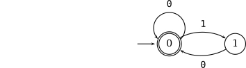
Figure 4.4 A DFA for the Swedish drinking protocol

The DFA in Figure 4.4 specifies legal sequences of activities according to the Swedish drinking protocol, where the state \(0\) is the start state and also the final state. The symbol 0 corresponds to drinking, whereas 1 corresponds to singing. That is, the sequence of activities must be a string of 0s and 1s accepted by the DFA.

The DFA d is initialized by

DFA::Transition t[] = {{0, 0, 0}, {0, 1, 1},
                       {1, 0, 0}, {-1, 0, 0}};
int f[] = {0,-1};
DFA d(0, t, f);

The array of transitions t is initialized by triples of integers (of type DFA::Transition). A triple \(\{a,s,b\}\) defines a transition from state \(a\) to state \(b\) with symbol \(s\). States are denoted by non-negative integers and symbols are integer values (as always, restricted to integer values that can be taken on by an integer variable, see Limits for integer values). A transition where \(a\) is \(-1\) marks the last transition in a transition array. The array of final states f lists all final states of the DFA, where the array is terminated by \(-1\). The first argument of the constructor of the DFA defines the start state.

Constraining an array of variables for four activities to the Swedish drinking protocol is done by

BoolVarArray x(home, 4, 0, 1);
extensional(home, x, d);

Note that the same DFA would also work with an array of integer variables.

The propagator for the extensional constraint is domain consistent and is based on [40].

Examples that use regular expressions for defining DFAs can be found in Regular expressions for extensional constraints.

Tuple sets (tables). Constraints can also be defined by a list of tuples, where each tuple defines one solution of the extensional constraint. For example, the following defines the Swedish drinking protocol for three activities by a list of tuples:

TupleSet t(3);
t.add(IntArgs({0,0,0}));
t.add(IntArgs({0,1,0}));
t.add(IntArgs({1,0,0}));
t.finalize();

Constraining an array of variables for three activities to the Swedish drinking protocol is done by

BoolVarArray x(home, 3, 0, 1);
extensional(home, x, t);

Note that before a tuple set can be used by a post function, it must be finalized as shown above. If a not-yet finalized tuple set is used for posting a constraint, an exception of type Int::NotYetFinalized is thrown.

The above example can be written more concisely as:

TupleSet t(3);
t.add({0,0,0}).add({0,1,0}).add({1,0,0})
 .finalize();

A tuple set can also be used as a negative tuple set, expressing that the tuples in the table are not allowed. For example, the following expresses that three activities do not follow the Swedish drinking protocol:

BoolVarArray x(home, 3, 0, 1);
extensional(home, x, false, t);

Note that extensional(home, x, t) abbreviates extensional(home, x, true, t). Extensional constraints using tuple sets also support reification. For example,

BoolVarArray x(home, 3, 0, 1);
BoolVar b(home, 0, 1)
extensional(home, x, t, b);

constrains b to one, if and only if the drinking activities comply with the Swedish drinking protocol.

Tuple sets can also be initialized by specifying their arity and a DFA. Hence, if d refers to the DFA for the Swedish drinking protocol, the above example can also be written as:

TupleSet t(3,d);

Tip 4.10 (When to use tuple sets rather than DFAs).

If a DFA is small and the arity is small, then it is typically more efficient to create a tuple set from the DFA and use it instead with an extensional constraint. However, if the arity is large or the DFA encodes many different tuples, it is typically more efficient to use the DFA directly.

◄

The propagators for the extensional constraint are domain consistent and are based on [13, 23, 63]. (see also GCCat: in_relation).

For several examples of extensional constraints using tuple sets, see Kakuro, Black hole patience, and Kakuro.

4.4.14. Sorted constraints

Sorted constraints relate an integer variable array to an array obtained by sorting the array. For example,

sorted(home, x, y);

constrains y to be x (of same size) sorted in increasing order. The more general variant features an additional integer variable array (again, of same size) z as in

sorted(home, x, y, z);

where z defines the sorting permutation, that is

\[\mathtt{x}_i=\mathtt{y}_{\mathtt{z}_i} \qquad\mbox{for }0\leq i<|\mathtt x|\]

The propagator for sorted is bounds consistent and is based on [35] (see also GCCat: sort, sort_permutation).

4.4.15. Bin-packing constraints

Bin packing constraints constrain how items can be packed into bins.

Single-dimensional bin-packing constraints. The bin-packing constraint is posted as

binpacking(home, l, b, s);

where l is an array of integer variables (the load variables), b is an array of integer variables (the bin variables), and s is an array of non-negative integers (the item sizes).

The load variables l determine the load \(\mathtt{l}_j\) of each bin \(j\) (\(0\leq j<|\mathtt{l}|\)) and the bin variables b determine for each item \(i\) (\(0\leq i<|\mathtt{b}|\)) into which bin \(\mathtt{b}_i\) it is packed. The size of an item \(i\) (\(0\leq i<|\mathtt{b}|\)) is defined by its item size \(\mathtt{s}_i\). Naturally, the number of bin variables and item sizes must coincide (\(|\mathtt{b}|=|\mathtt{s}|\)).

The bin-packing constraint enforces that all items are packed into bins

\[\mathtt{b}_i\in\{0,\ldots,|\mathtt{l}|-1\} \qquad\mbox{for }0\leq i<|\mathtt{b}|\]

and that the load of each bin corresponds to the items packed into it

\[\mathtt{l}_j=\sum_{\{i\in\{0,\ldots,|\mathtt{b}|-1\}\mid\mathtt{b}_j=i\}} \mathtt{s}_i \qquad\mbox{for }0\leq j<|\mathtt{l}|\]

The constraint is implemented by the propagator introduced in [56] (see also GCCat: bin_packing, bin_packing_capa). For an example using the bin-packing constraint and CDBF (complete decreasing best fit) [17] as a specialized branching for bin-packing, see Bin packing and Bin packing.

Multi-dimensional bin-packing constraints. The multi-dimensional bin-packing constraint is posted as

binpacking(home, d, l, b, s, c);

where d is a positive integer (the dimension), l is an array of integer variables (the load variables), b is an array of integer variables (the bin variables), s is an array of non-negative integers (the item sizes), and c is an array of non-negative integers (the bin capacities).

In the following \(n\) refers to the number of items and \(m\) refers to the number of bins. The bin variables b determine for each item \(i\) (\(0\leq i<n\)) into which bin \(\mathtt{b}_i\) it is packed. The load variables l determine the load \(\mathtt{l}_{j\cdot \mathtt{d} + k}\) for each bin \(j\) (\(0\leq j<m\)) and dimension \(k\) (\(0\leq k<\mathtt{d}\)). The size of an item \(i\) (\(0\leq i<n\)) in dimension \(k\) (\(0\leq k<\mathtt{d}\)) is defined by the item size \(\mathtt{s}_{i\cdot\mathtt{d} + k}\). The capacity of all bins \(j\) (\(0\leq j<m)\) in dimension \(k\) (\(0\leq k<\mathtt{d}\)) is defined by \(\mathtt{c}_k\). Naturally, the number of bin variables, load variables, item sizes, and capacities must satisfy that \(|\mathtt{b}|=n\), \(|\mathtt{l}|=m\cdot\mathtt{d}\), \(|\mathtt{s}|=n\cdot\mathtt{d}\), and \(|\mathtt{c}|=\mathtt{d}\).

The multi-dimensional bin-packing constraint enforces that all items are packed into bins

\[\mathtt{b}_i\in\{0,\ldots,m-1\} \qquad\mbox{for }0\leq i<n\]

and that the load of each bin corresponds to the items packed into it for each dimension

\[\mathtt{l}_{j\cdot \mathtt{d} + k} = \sum_{\{i\in\{0,\ldots,n-1\}\mid\mathtt{b}_{j\cdot\mathtt{d}+k}=i\}}\mathtt{s}_{i\cdot\mathtt{d}+k} \qquad\mbox{for }0\leq j<m, 0\leq k<\mathtt{d}\]

Furthermore, the load variables must satisfy the capacity constraints

\[\mathtt{l}_{j\cdot \mathtt{d} + k} \leq \mathtt{c}_k \qquad\mbox{for }0\leq j<m, 0\leq k<\mathtt{d}\]

In addition to posting propagators, the post function

IntSet m = binpacking(home, d, l, b, s, c);

returns an integer set m of type IntSet. The set m contains a maximal number of conflicting items that must be packed into pairwise distinct bins where the items are chosen to maximize the conflict with other items. This information can be used for symmetry breaking.

Important

Posting the constraint (not propagating it) has exponential complexity in the number of items. This is due to the use of the Bron-Kerbosch algorithm [9, 10] for finding all sets of conflicting items.

The constraint is implemented by the decomposition introduced in [21] using a single-dimensional bin-packing constraint for each dimension together with derived constraints capturing capacity conflicts. For an example using the multi-dimensional bin-packing constraint see Multi-dimensional bin packing.

4.4.16. Geometrical packing constraints

Geometrical packing constraints constrain how rectangles can be packed such that no two rectangles from a collection of rectangles overlap.

If x and y are integer variable arrays and w and h are integer arrays (where all arrays must be of the same size), then

nooverlap(home, x, w, y, h);

propagates that the rectangles defined by coordinates \(\langle \mathtt x_i,\mathtt y_i\rangle\), widths \(\mathtt w_i\), and heights \(\mathtt h_i\) for \(0\leq i<|\mathtt x|\) do not overlap. That is, the following constraint is enforced (see also Boolean expressions and relations for a picture):

\[\left(\mathtt{x}_i+\mathtt{w}_i\leq \mathtt{x}_j\right) \vee \left(\mathtt{x}_j+\mathtt{w}_j\leq \mathtt{x}_i\right) \vee \left(\mathtt{y}_i+\mathtt{h}_i\leq \mathtt{y}_j\right) \vee \left(\mathtt{y}_j+\mathtt{h}_j\leq \mathtt{y}_i\right)\]

Note that the width or the height of a rectangle can be zero. In this case, the rectangle does not occupy any space. However no other rectangle is allowed to be placed where the zero-sized rectangle is placed.

Rectangles can also be modeled as optional through a Boolean variable \(\mathtt m_i\) for each rectangle \(i\). If the Boolean variable \(\mathtt{m}_i\) is 1 the rectangle is mandatory and considered by the packing constraint, if it is 0, the rectangle is ignored.

With an array of Boolean variables m the constraint taking optional rectangles into account is posted by

nooverlap(home, x, w, y, h, m);

The arrays defining the dimensions (that is, w and h for rectangles) can also be arrays of integer variables, where its values are constrained to be non-negative. In this case, the constraint post functions expects both a start and end coordinate. That is, by posting

nooverlap(home, x0, w, x1, y0, h, y1);

it is enforced that the rectangles defined by the start coordinate \(\langle \mathtt{x0}_i,\mathtt{y0}_i\rangle\), the dimension \(\langle \mathtt{w}_i,\mathtt{h}_i\rangle\), and the end coordinate \(\langle \mathtt{x1}_i,\mathtt{y1}_i\rangle\) do not overlap. The end coordinates are not constrained to be the sum of the start coordinates and dimensions. That is, one has to explicitly post the linear constraints such that

\[\left(\mathtt{x0}_i+\mathtt{w}_i=\mathtt{x1}_i\right)\wedge \left(\mathtt{y0}_i+\mathtt{h}_i=\mathtt{y1}_i\right)\]

The constraints are implemented by a naive propagator (considering pairwise no-overlap between rectangles including constructive disjunction, see also GCCat: diffn), this will change in the future. For an example using the no-overlap constraint, see Packing squares into a rectangle.

4.4.17. Circuit and Hamiltonian path constraints

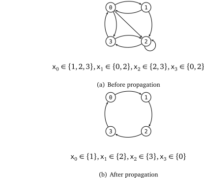
Figure 4.5 Representing edges and propagating circuit

The circuit and path constraints (see Graph constraints) use values of variables in an integer variable array x as edges: if \(j\in\mathtt{x}_i\), the corresponding graph contains the edge \(i\to j\) for \(0\leq i,j<|\mathtt{x}|\). Obviously, the graph has the nodes \(0\) to \(|\mathtt{x}|-1\).

Circuit constraints. Assume that x is an integer variable array (circuit does not support Boolean variables). Then,

circuit(home, x);

constrains the values of x such that their corresponding edges form a Hamiltonian circuit (see also GCCat: circuit). For an example before and after propagation of circuit see Figure 4.5. For an example, see Knight’s tour and n-Knights tour (model using circuit).

Common applications of circuit also require costs for the edges in the graph. Assume that the cost for an edge \(i\to j\) from node \(i\) to node \(j\) is defined by the following matrix:

\[\begin{array}{|c|rrrr|} \hline i\to j&\cdot\to 0&\cdot\to 1&\cdot\to 2&\cdot\to 3\\ \hline 0\to\cdot & 0 & 3 & 5 & 7\\ 1\to\cdot & 4 & 0 & 9 & 6\\ 2\to\cdot & 2 & 1 & 0 & 5\\ 3\to\cdot & -7 & 8 & -2 & 0\\ \hline \end{array}\]

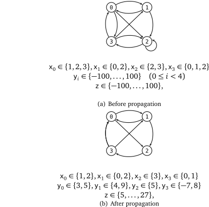
Figure 4.6 Representing edges and propagating circuit with cost

Then, by

IntArgs c({ 0, 3, 5, 7,
            4, 0, 9, 6,
            2, 1, 0, 5,
           -7, 8,-2, 0});
circuit(home, c, x, y, z);

the integer variables x are constrained to the values forming the circuit as above, while the integer variables y define the cost of the edge for each node (these variables can be omitted), and the integer variable z defines the total cost of the edges in the circuit. Note that the matrix interface as described in Matrix interface for arrays might come in handy for setting up the cost matrix.

Figure 4.6 shows a simple example for propagation circuit with cost where the cost matrix from above is used. For an example, see Travelling salesman problem (TSP).

Hamiltonian path constraints. The path constraint (see Graph constraints) is similar to the circuit constraint and enforces that nodes in a graph from a Hamiltonian path. Assume that x is an integer variable array (path does not support Boolean variables) and s (for start) and e (for end) are integer variables. Then,

path(home, x, s, e);

constrains the values of x, s, and e such that their corresponding edges form a Hamiltonian path that starts at node \(\mathtt{x}_{\mathtt{s}}\) and ends at node \(\mathtt{x}_{\mathtt{e}}\) (the value of the variable \(\mathtt{x}_{\mathtt{e}}\) is always \(|\mathtt{x}|\)).

As an example, assume that the integer variable array x has three elements (that is, \(|\mathtt{x}|=3\)) with values between \(0\) and \(3\). Then all solutions to

path(home, x, s, e);

are as follows:

x	s	e
\(\langle\mathtt 1, \mathtt 2, \mathtt 3\rangle\)	\(\mathtt 0\)	\(\mathtt 2\)
\(\langle\mathtt 1, \mathtt 3, \mathtt 0\rangle\)	\(\mathtt 2\)	\(\mathtt 1\)
\(\langle\mathtt 2, \mathtt 0, \mathtt 3\rangle\)	\(\mathtt 1\)	\(\mathtt 2\)
\(\langle\mathtt 2, \mathtt 3, \mathtt 1\rangle\)	\(\mathtt 0\)	\(\mathtt 1\)
\(\langle\mathtt 3, \mathtt 0, \mathtt 1\rangle\)	\(\mathtt 2\)	\(\mathtt 0\)
\(\langle\mathtt 3, \mathtt 2, \mathtt 0\rangle\)	\(\mathtt 1\)	\(\mathtt 0\)

The path constraint provides, similar to circuit, variants for costs for edges in a Hamiltonian path, see Graph constraints.

4.4.18. Scheduling constraints

This section provides an overview of scheduling constraints.

4.4.18.1. Unary resource constraints

A unary resource constraint models that a number of tasks to be executed on a single resource do not overlap, where each task is defined by its start time (an integer variable), its duration (an integer or integer variable), and possibly its end time (if the duration is a variable). Unary resource constraints are also known as disjunctive scheduling constraints.

For example, assume that four tasks with durations 2, 7, 4, and 11 are to be executed on the same resource where the start times are specified by an array of integer variables (of course, with four variables). Then, posting

IntArgs d({2,7,4,11});
unary(home, s, d);

constrains the start times in s such that the execution of none of the tasks overlaps in time (see Scheduling constraints) (see also GCCat: disjunctive).

Tip 4.11 (Tasks with duration zero).

Tasks with duration zero are still useful for modeling: even though they do not take any time to be executed on the resource, they prevent that any other task can run at the same time.

◄

Selecting the propagation level. All propagators implementing unary perform overload-checking. The propagators can be posted offering basic or advanced propagation, where basic propagation only is the default. Basic propagation is selected if the constraint is posted with an additional integer propagation level argument (see Selecting the propagation level) as

unary(home, s, d, IPL_BASIC);

Basic propagation performs time-tabling, see for example [2], in addition to overload checking.

Advanced propagation is selected by

unary(home, s, d, IPL_ADVANCED);

and performs overload-checking, detectable precedences, not-first-not-last, and edge-finding, following [66].

Basic and advanced propagation can be combined by

unary(home, s, d, IPL_BASIC_ADVANCED);

which is more convenient than the equivalent

unary(home, s, d, 
      static_cast<IntPropLevel>(IPL_BASIC | IPL_ADVANCED));

It performs time-tabling in addition to the advanced algorithms.

All algorithms require \(O(n \log n)\) runtime for \(n\) tasks, however basic propagation is more efficient than advanced propagation.

Optional tasks. A common variant for unary resource constraints is where tasks can be optional: each task \(t\) has a Boolean variable \(b\) attached to it. If \(b=1\) then the task is mandatory and is scheduled on the resource. If \(b=0\) then the task is excluded and is not scheduled. Otherwise, the task is said to be optional. Assume that b refers to an array of Boolean variables also of size 4, then

IntArgs d({2,7,4,11});
unary(home, s, d, b);

posts a propagator that constrains the start times s (of course, only if a task is mandatory) as well the Boolean variables in b (if a task becomes excluded as otherwise no feasible schedule would exist).

Tasks with flexible duration. The duration of a task can also be given as an integer variable instead of a constant integer. In this case, we say that the tasks are flexible. In addition to the flexible duration, the unary constraint also requires variables for the end time of each task.

Given variable arrays s, d, and e for the start times, durations, and end times, a unary resource constraint is posted as

unary(home, s, d, e);

However, the additional constraint for each task \(i\) that \(\texttt{s}[i]+\texttt{d}[i]=\texttt{e}[i]\) is not enforced automatically. Therefore, a model typically must contain additional constraints like

for (int i=0; i<s.size(); i++)
  post(home, s[i]+d[i]==e[i]);

The unary post function also exists in a variant with flexible, optional tasks.

4.4.18.2. Cumulative scheduling constraints

Gecode provides two generalizations of the unary resource scheduling constraint. The first one, called cumulative, models a resource where tasks can overlap. The resource has a limited capacity, and each task requires a certain resource usage. At each point in time, the sum of the resource usages of all tasks running at that point must not exceed the capacity. The second generalization, called cumulatives, deals with several cumulative resources at once.

Cumulative single-resource constraint. The single-resource constraint cumulative has nearly the same interface as unary. The only difference is a parameter c specifying the resource capacity, and an additional integer array u for the resource usage of each task. Assuming that s and d give the start times and durations as before, the following models a resource where two tasks can overlap, and the first three tasks require one unit of the resource, while the last task requires two:

IntArgs u({1,1,1,2});
cumulative(home, 2, s, d, u);

The capacity can be an integer variable or a nonnegative integer. The resource usage must be strictly positive. As for unary, there exist versions with optional, flexible, and flexible and optional tasks.

The propagators implementing the cumulative constraint always perform overload checking [65]. Basic propagation performs time-tabling, see for example [2], and can be selected by giving IPL_BASIC as additional integer propagation level argument. The cost of basic propagation is \(O(n\log n)\) for \(n\) tasks. Advanced propagation (selected by IPL_ADVANCED) performs edge-finding [64] (see also GCCat: cumulative). The cost of advanced propagation is \(O(kn\log n)\) for \(n\) tasks where \(k\) is the number of different resource usage values. Basic and advanced propagation can be combined as described in Unary resource constraints.

Cumulative multi-resource constraint. Given a set of resources that have some specified usage limit and a set of tasks that must be placed on these resources according to start-times, durations, resource usage, and resource compatibility, the cumulatives constraint (see Scheduling constraints) can be used for the placement of these tasks. The limit for the resources can be either a maximum or a minimum, and the resource usage of a task can be positive, negative, or zero. The limit is only valid over the intervals where there is at least one task assigned on that particular resource.

Consider the following code.

cumulatives(home, resource, start, duration, end, height, 
            limit, atmost);

This code posts a constraint over a set of tasks \(T\), where each task \(T_i\) is defined by \(\langle \mathtt{resource}_i, \mathtt{start}_i, \mathtt{duration}_i, \mathtt{end}_i, \mathtt{height}_i \rangle\). The resource component indicates the potential resources that the task can use; start, duration, and end indicate when the task can occur; and finally the height component indicates the amount of resource the task uses (or “provides” in the case of a negative value). The resource \(R_i\) is defined by the limit \(\mathtt{limit}_i\) and the parameter atmost. The latter is common for all resources, and indicates whether the limits are maximum limits (atmost is true) or minimum limits (atmost is false).

As for flexible tasks in Unary resource constraints, the cumulatives constraint does not enforce that \(\mathtt{start}_i+\mathtt{duration}_i=\mathtt{end}_i\). This additional constraint must be posted manually.

The parameters start and end are always integer variable arrays; resource, duration, and height can be either integer variable arrays or integer arrays; and limit is always an array of integers.

For an example using cumulatives see Packing squares into a rectangle, where the cumulatives constraints is used to model packing a set of squares. For an insightful discussion of how to use cumulatives for modeling, see [5] (the propagator for cumulative is implemented following this paper, see also GCCat: cumulatives).

4.4.19. Value precedence constraints

Value precedence constraints over integer variables enforce that a value precedes another value in an array of integer variables. By

precede(home, x, s, t);

where x is an array of integer variables and both s and t are integers, the following is enforced: if there exists \(j\) (\(0\leq j<|\mathtt{x}|\)) such that \(\mathtt{x}_j=\mathtt{t}\), then there must exist \(i\) with \(i<j\) such that \(\mathtt{x}_i=\mathtt{s}\). This is equivalent to:

1. \(\mathtt{x}_0 \neq \mathtt t\), and

2. if \(\mathtt{x}_j=\mathtt t\) then \(\bigvee_{i=0}^{j-1} \mathtt{x}_i=\mathtt s\) for \(1\leq j<|\mathtt x|\).

A generalization is available for precedences between several integer values. By

precede(home, x, c);

where x is an array of integer variables and c is an array of integers, it is enforced that \(\mathtt{c}_i\) precedes \(\mathtt{c}_{i+1}\) in x for \(0\leq i<|\mathtt c|-1\). That is

1. \(\mathtt{x}_0 \neq \mathtt{c}_{k+1}\) for \(0\leq k<|\mathtt{c}|-1\), and

2. if \(\mathtt{x}_j=\mathtt{c}_{k+1}\) then \(\bigvee_{i=0}^{j-1} \mathtt{x}_i=\mathtt{c}_k\) for \(1\leq j<|\mathtt x|\) and \(0\leq k<|\mathtt{c}|-1\).

The constraint is implemented by the domain consistent propagator introduced in [27] (see also GCCat: int_value_precede, int_value_precede_chain), the paper also explains how to use the precede constraint for breaking value symmetries. For an example, see Schur’s lemma.

4.5. Synchronized execution

Gecode offers support in Synchronized execution for executing a function (any function that is compatible with the type std::function) when integer or Boolean variables become assigned.

The following code

wait(home, x, [] (Space& home) { ...; });

posts a propagator that waits until the integer or Boolean variable x (or, if x is an array of variables: all variables in x) is assigned. If x becomes assigned, the function passed as argument is executed with the current home space passed as argument. The type of the function must be

  std::function<void(Space& home)>

Tip 4.12 (Failing a space).

If you want to fail a space home (for example when executing a continuation function as discussed above), you can do that by

home.fail();

◄

The following code

when(home, x,
     [] (Space& home) { ...; },
     [] (Space& home) { ...; });

creates a propagator that will be run exactly once when the Boolean variable x becomes assigned. If x becomes assigned to 1, the first function is executed. If x becomes assigned to 0, the second function is executed. Both functions get the current home space of the propagator passed as argument and must be of type

  std::function<void(Space& home)>

The else-function is optional and can be omitted.

[1]

Actually, if an argument array has few fields it uses some space that is part of the object implementing the array rather than allocating memory from the heap. Hence, small argument arrays reside entirely on the stack.